rounD (LevelX)¶

About¶

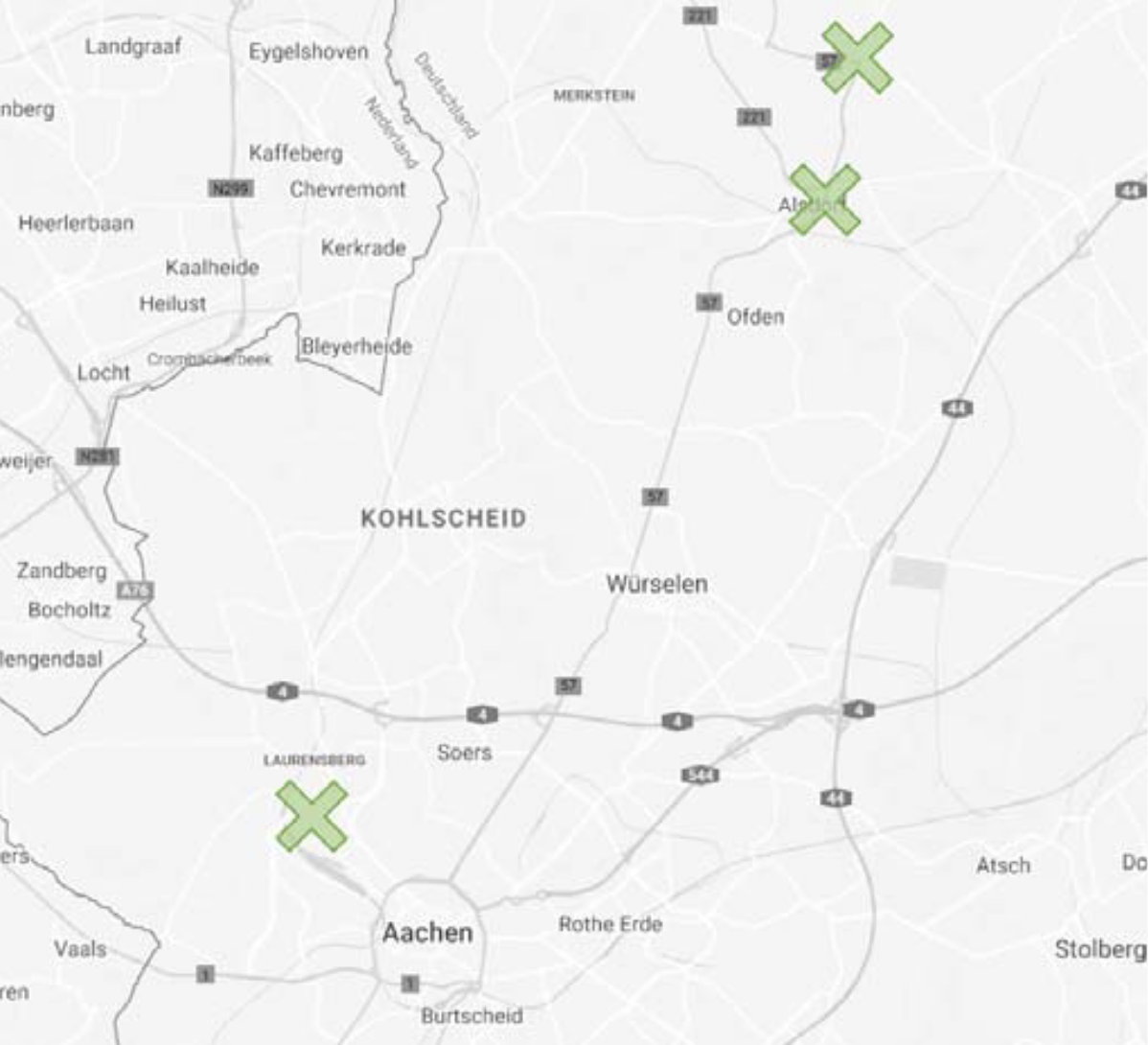
The rounD dataset was created and published by a team from the Institute for Automotive Engineering (ika) of RWTH Aachen University to promote research in many different domains of mobility. The dataset can therefore be downloaded and used free of charge for academic and research purposes.

This dataset contains a total of six hours of recordings with more than 13,746 road users including cars, vans, trucks, buses, pedestrians, bicycles and motorcycles from three roundabouts.

How to Apply Dataset¶

The rounD dataset is free for non-commercial use only. According to the license and protocols, as a third-party, we cannot share any form of this dataset online. Please visit the official website of rounD, fill in the application form and send your request.

The maps of rounD dataset are manually created by Tactics2D, in the format of OpenStreetMap (OSM), labeled in Lanelet2 style. The maps are stored in data/rounD_map. You can download them from here

Citation¶

@inproceedings{rounD,
    title={The rounD Dataset: A Drone Dataset of Road User Trajectories at Roundabouts in Germany},
    author={Krajewski, Robert and Moers, Tobias and Bock, Julian and Vater, Lennart and Eckstein, Lutz},
    booktitle={2020 IEEE 23rd International Conference on Intelligent Transportation Systems (ITSC)},
    pages={1-6},
    year={2020},
    doi={10.1109/ITSC45102.2020.9294728}
}

Data Analysis¶

This part is independently conducted by Tactics2D.

According to meta records:

• Trajectory data files 00 are recorded in location 1 (denoted as rounD_1)
• Trajectory data files 01 are recorded in location 2 (denoted as rounD_2)
• Trajectory data files 03-23 are recorded in location 0 (denoted as rounD_0). Among them, files 03-08 are recorded in region 0 and files 09-23 are recorded in region 1.

In [1]:

hide_input

%matplotlib inline
import warnings

warnings.filterwarnings("ignore")

import logging

logging.basicConfig(level=logging.WARNING)

import pandas as pd
import polars as pl
import numpy as np
import matplotlib as mpl
import matplotlib.gridspec as gridspec
import matplotlib.pyplot as plt
import seaborn as sns

%matplotlib inline import warnings warnings.filterwarnings("ignore") import logging logging.basicConfig(level=logging.WARNING) import pandas as pd import polars as pl import numpy as np import matplotlib as mpl import matplotlib.gridspec as gridspec import matplotlib.pyplot as plt import seaborn as sns

In [2]:

hide_input

# Setting up parameters for matplotlib
mpl.rcParams.update(
    {
        "figure.dpi": 200,  # 200 for high quality
        "font.family": "DejaVu Sans Mono",
        "font.size": 6,
        "font.stretch": "semi-expanded",
        "animation.html": "jshtml",
        "animation.embed_limit": 5000,
        "axes.edgecolor": "black",
        "axes.linewidth": 0.8,
        "axes.grid": True,
        "grid.color": "#cccccc",
        "axes.facecolor": "white",
    }
)
sns.set_palette("Set2")

# Setting up parameters for matplotlib mpl.rcParams.update( { "figure.dpi": 200, # 200 for high quality "font.family": "DejaVu Sans Mono", "font.size": 6, "font.stretch": "semi-expanded", "animation.html": "jshtml", "animation.embed_limit": 5000, "axes.edgecolor": "black", "axes.linewidth": 0.8, "axes.grid": True, "grid.color": "#cccccc", "axes.facecolor": "white", } ) sns.set_palette("Set2")

In [3]:

hide_input

locations = dict()
dfs_meta = pd.DataFrame()
for i in range(24):
    df_meta = pd.read_csv("../../data/rounD/data/%02d_recordingMeta.csv" % i)
    locations[i] = df_meta["locationId"][0]
    dfs_meta = pd.concat([dfs_meta, df_meta], ignore_index=True)

locations = dict() dfs_meta = pd.DataFrame() for i in range(24): df_meta = pd.read_csv("../../data/rounD/data/%02d_recordingMeta.csv" % i) locations[i] = df_meta["locationId"][0] dfs_meta = pd.concat([dfs_meta, df_meta], ignore_index=True)

In [4]:

hide_input

dfs_track_meta = pd.DataFrame()
for i in range(24):
    df_track_meta = pd.read_csv("../../data/rounD/data/%02d_tracksMeta.csv" % i)
    df_track_meta["locationId"] = locations[i]
    df_track_meta["fileId"] = i
    dfs_track_meta = pd.concat([dfs_track_meta, df_track_meta], ignore_index=True)

dfs_track_meta = pd.DataFrame() for i in range(24): df_track_meta = pd.read_csv("../../data/rounD/data/%02d_tracksMeta.csv" % i) df_track_meta["locationId"] = locations[i] df_track_meta["fileId"] = i dfs_track_meta = pd.concat([dfs_track_meta, df_track_meta], ignore_index=True)

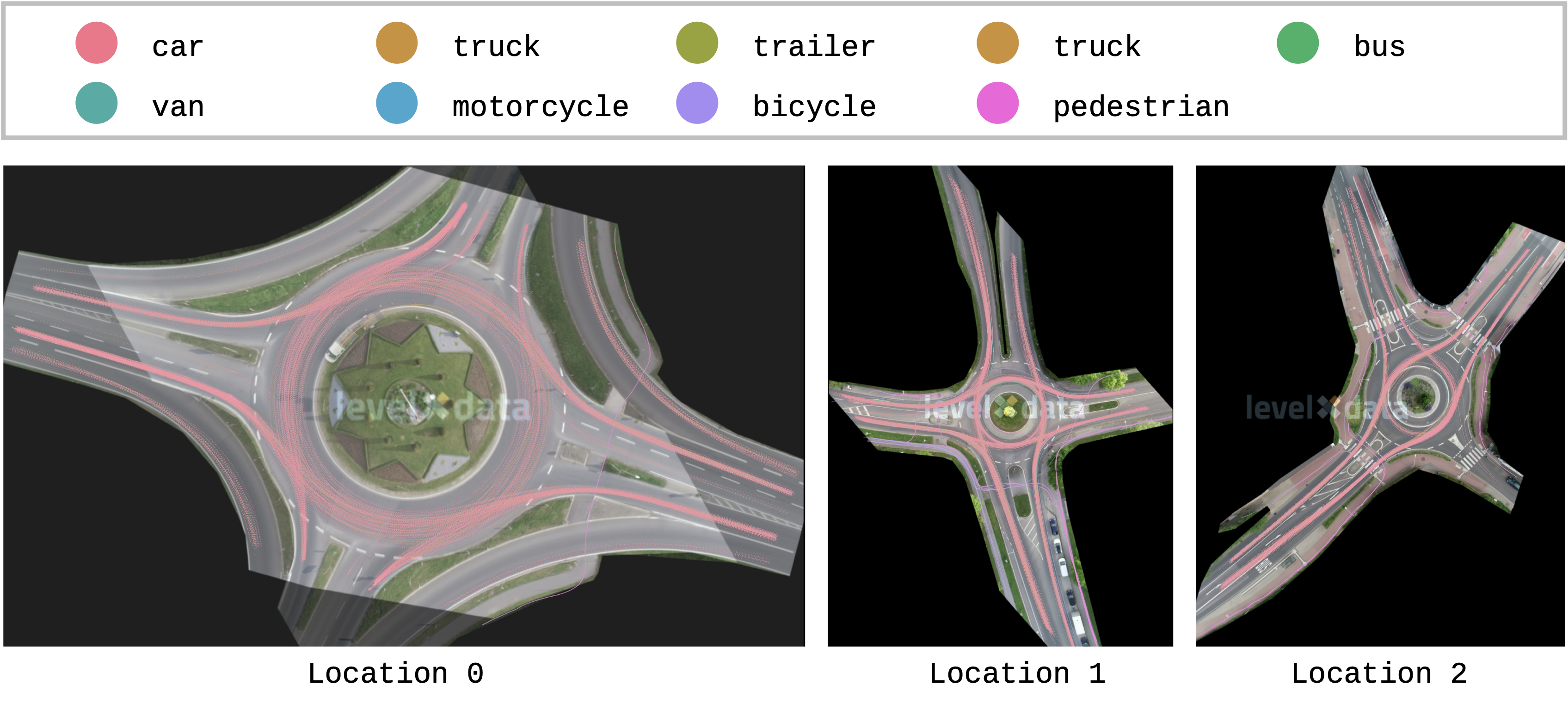
Distribution of Trajectory on Map¶

The projection of trajectories onto the map reveals that the majority of road users in the rounD dataset are cars. The vehicle trajectories exhibit behavior that aligns with typical driving patterns.

Distribution of Trajectory Categories¶

The distribution of trajectory categories exhibits substantial variation across different locations. At a single location, the proportion of vehicle trajectories also fluctuates over time or between samples.

In [5]:

hide_input

dfs = [pl.DataFrame()] * 3

for i in range(24):
    df = pl.read_csv("../../data/rounD/data/%02d_tracks.csv" % i)
    df = df.select(["trackId", "frame", "xCenter", "yCenter", "heading", "xVelocity", "yVelocity"])
    df = df.with_columns(pl.lit(i).alias("fileId"))
    df = df.join(
        pl.DataFrame(dfs_track_meta)[["fileId", "trackId", "class"]],
        on=["fileId", "trackId"],
        how="left",
    )

    dfs[locations[i]] = pl.concat([dfs[locations[i]], df])

dfs = [pl.DataFrame()] * 3 for i in range(24): df = pl.read_csv("../../data/rounD/data/%02d_tracks.csv" % i) df = df.select(["trackId", "frame", "xCenter", "yCenter", "heading", "xVelocity", "yVelocity"]) df = df.with_columns(pl.lit(i).alias("fileId")) df = df.join( pl.DataFrame(dfs_track_meta)[["fileId", "trackId", "class"]], on=["fileId", "trackId"], how="left", ) dfs[locations[i]] = pl.concat([dfs[locations[i]], df])

In [6]:

hide_input

for i in range(3):
    x_min = np.floor(dfs[i]["xCenter"].min())
    x_max = np.ceil(dfs[i]["xCenter"].max())
    y_min = np.floor((-dfs[i]["yCenter"]).min())
    y_max = np.ceil((-dfs[i]["yCenter"]).max())
    vx = dfs[i]["xVelocity"].to_numpy()
    vy = dfs[i]["yVelocity"].to_numpy()

    x_edges = np.linspace(x_min, x_max, num=int((x_max - x_min) * 10 + 1), endpoint=True)
    y_edges = np.linspace(y_min, y_max, num=int((y_max - y_min) * 10 + 1), endpoint=True)
    x_bin = np.digitize(dfs[i]["xCenter"].to_numpy(), x_edges) - 1
    y_bin = np.digitize((-dfs[i]["yCenter"]).to_numpy(), y_edges) - 1
    speed = np.sqrt(vx**2 + vy**2)

    dfs[i] = dfs[i].with_columns(
        [pl.Series("x_bin", x_bin), pl.Series("y_bin", y_bin), pl.Series("speed (m/s)", speed)]
    )

for i in range(3): x_min = np.floor(dfs[i]["xCenter"].min()) x_max = np.ceil(dfs[i]["xCenter"].max()) y_min = np.floor((-dfs[i]["yCenter"]).min()) y_max = np.ceil((-dfs[i]["yCenter"]).max()) vx = dfs[i]["xVelocity"].to_numpy() vy = dfs[i]["yVelocity"].to_numpy() x_edges = np.linspace(x_min, x_max, num=int((x_max - x_min) * 10 + 1), endpoint=True) y_edges = np.linspace(y_min, y_max, num=int((y_max - y_min) * 10 + 1), endpoint=True) x_bin = np.digitize(dfs[i]["xCenter"].to_numpy(), x_edges) - 1 y_bin = np.digitize((-dfs[i]["yCenter"]).to_numpy(), y_edges) - 1 speed = np.sqrt(vx**2 + vy**2) dfs[i] = dfs[i].with_columns( [pl.Series("x_bin", x_bin), pl.Series("y_bin", y_bin), pl.Series("speed (m/s)", speed)] )

In [7]:

hide_input

dfs_meta["vehicle_ratio"] = dfs_meta["numVehicles"] / dfs_meta["numTracks"]
dfs_meta["locationId"] = pd.Categorical(dfs_meta["locationId"], categories=[0, 1, 2], ordered=True)

dfs_meta["vehicle_ratio"] = dfs_meta["numVehicles"] / dfs_meta["numTracks"] dfs_meta["locationId"] = pd.Categorical(dfs_meta["locationId"], categories=[0, 1, 2], ordered=True)

In [8]:

hide_input

f, ax = plt.subplots(figsize=(6, 3))

sns.boxplot(data=dfs_meta, x="vehicle_ratio", y="locationId", width=0.5, ax=ax)

sns.stripplot(data=dfs_meta, x="vehicle_ratio", y="locationId", alpha=0.6, ax=ax)

ax.set_xticks([0.9, 1.0])
ax.set_xticklabels(["90", "100"])
ax.yaxis.grid(True)
ax.set_xlabel(
    "Proportion of all types of vehicles (`car`, `truck_bus`, \n`trailer`, `bus`, and 'van`) in each file (%)"
)
ax.set_ylabel("Location")
plt.show()

f, ax = plt.subplots(figsize=(6, 3)) sns.boxplot(data=dfs_meta, x="vehicle_ratio", y="locationId", width=0.5, ax=ax) sns.stripplot(data=dfs_meta, x="vehicle_ratio", y="locationId", alpha=0.6, ax=ax) ax.set_xticks([0.9, 1.0]) ax.set_xticklabels(["90", "100"]) ax.yaxis.grid(True) ax.set_xlabel( "Proportion of all types of vehicles (`car`, `truck_bus`, \n`trailer`, `bus`, and 'van`) in each file (%)" ) ax.set_ylabel("Location") plt.show()

Distribution of Average Speed on Map¶

The average speed in the roundabout scenario is higher than at intersections but lower than on highways. Before entering the roundabout, vehicles typically travel at an average speed of around 15 m/s (54 km/h). Once inside the roundabout, the speed decreases to approximately 7.5 m/s (27 km/h). The lowest speeds are observed at the entry points, indicating significant deceleration, while vehicles tend to accelerate again upon exiting the roundabout.

In [9]:

hide_input

fig = plt.figure(figsize=(6, 3))
gs = gridspec.GridSpec(1, 3, figure=fig, width_ratios=[1.17, 0.65, 0.76])

axes = []
for i in range(3):
    ax = fig.add_subplot(gs[0, i])
    df_speed_heatmap = (
        dfs[i]
        .group_by(["y_bin", "x_bin"])
        .agg(pl.col("speed (m/s)").mean().alias("avg_speed"))
        .sort(["y_bin", "x_bin"])
    ).to_pandas()
    grid = df_speed_heatmap.pivot(index="y_bin", columns="x_bin", values="avg_speed")
    hm = sns.heatmap(
        grid, ax=ax, cmap="cool", cbar=False, xticklabels=False, yticklabels=False, vmin=0, vmax=20
    )

    ax.set_aspect("equal")
    ax.set_xlabel(f"Location {i}", rotation=0)
    ax.set_ylabel("")

    axes.append(ax)

cbar_ax = fig.add_axes([0.1, 0.94, 0.8, 0.02])
cbar = fig.colorbar(hm.get_children()[0], cax=cbar_ax, orientation="horizontal")

plt.tight_layout(rect=[0.0, 0.0, 1, 0.92])
plt.show()

fig = plt.figure(figsize=(6, 3)) gs = gridspec.GridSpec(1, 3, figure=fig, width_ratios=[1.17, 0.65, 0.76]) axes = [] for i in range(3): ax = fig.add_subplot(gs[0, i]) df_speed_heatmap = ( dfs[i] .group_by(["y_bin", "x_bin"]) .agg(pl.col("speed (m/s)").mean().alias("avg_speed")) .sort(["y_bin", "x_bin"]) ).to_pandas() grid = df_speed_heatmap.pivot(index="y_bin", columns="x_bin", values="avg_speed") hm = sns.heatmap( grid, ax=ax, cmap="cool", cbar=False, xticklabels=False, yticklabels=False, vmin=0, vmax=20 ) ax.set_aspect("equal") ax.set_xlabel(f"Location {i}", rotation=0) ax.set_ylabel("") axes.append(ax) cbar_ax = fig.add_axes([0.1, 0.94, 0.8, 0.02]) cbar = fig.colorbar(hm.get_children()[0], cax=cbar_ax, orientation="horizontal") plt.tight_layout(rect=[0.0, 0.0, 1, 0.92]) plt.show()

Distribution of Speed by Trajectory Type¶

The peak of the speed distribution differs across trajectory types. Cars consistently exhibit the highest speed peaks, while pedestrians show the lowest. Additionally, the peak speed for each type varies depending on the location.

In [10]:

hide_input

fig, axes = plt.subplots(3, 1, figsize=(6, 4), sharex=True)
for i in range(3):
    df_speed = dfs[i].to_pandas()

    sns.histplot(
        df_speed,
        x="speed (m/s)",
        hue="class",
        hue_order=["car", "truck", "trailer", "bus", "motorcycle", "bicycle", "pedestrian"],
        multiple="layer",
        palette="Set2",
        ax=axes[i],
        stat="density",
        common_norm=False,
        binwidth=0.25,
        binrange=(0, 25),
        linewidth=0,
        alpha=0.5,
        legend=(i == 0),
    )

    axes[i].set_xlim([0, 25])
    axes[i].set_ylabel(f"Location {i+1}")

fig.text(0.02, 0.5, "Probability Density", va="center", rotation="vertical")

fig.tight_layout(rect=[0.03, 0, 1, 1])
plt.show()

fig, axes = plt.subplots(3, 1, figsize=(6, 4), sharex=True) for i in range(3): df_speed = dfs[i].to_pandas() sns.histplot( df_speed, x="speed (m/s)", hue="class", hue_order=["car", "truck", "trailer", "bus", "motorcycle", "bicycle", "pedestrian"], multiple="layer", palette="Set2", ax=axes[i], stat="density", common_norm=False, binwidth=0.25, binrange=(0, 25), linewidth=0, alpha=0.5, legend=(i == 0), ) axes[i].set_xlim([0, 25]) axes[i].set_ylabel(f"Location {i+1}") fig.text(0.02, 0.5, "Probability Density", va="center", rotation="vertical") fig.tight_layout(rect=[0.03, 0, 1, 1]) plt.show()

Tactics2D Integration¶

This section explains how to parse and replay logs from the rounD dataset by Tactics2D.

Dataset Preparation¶

You can place the rounD dataset in any directory of your choice. However, it’s important to maintain the following folder structure for compatibility:

rounD
├── data
│   ├── 01_highway.png
│   ├── 01_recordingMeta.csv
│   ├── 01_tracks.csv
│   ├── 01_tracksMeta.csv
│   ├── ...

Class Mapping¶

The table below illustrates how classes from the rounD dataset are mapped to corresponding traffic participants in the Tactics2D framework.

Class	Tactics2D
car	tactics2d.participant.element.Vehicle
truck	tactics2d.participant.element.Vehicle
trailer	tactics2d.participant.element.Vehicle
bus	tactics2d.participant.element.Vehicle
motorcycle	tactics2d.participant.element.Cyclist
bicycle	tactics2d.participant.element.Cyclist
pedestrian	tactics2d.participant.element.Pedestrian

Parse and Replay Logs¶

To parse, replay, and visualize the rounD dataset using Tactics2D, you can use the following code snippet:

In [11]:

%matplotlib notebook

import os
import numpy as np
from matplotlib.animation import FuncAnimation
from shapely.geometry import Point
from IPython.display import HTML

from tactics2d.dataset_parser import LevelXParser
from tactics2d.map.parser import OSMParser
from tactics2d.map.map_config import ROUND_MAP_CONFIG
from tactics2d.sensor import BEVCamera
from tactics2d.renderer import MatplotlibRenderer

%matplotlib notebook import os import numpy as np from matplotlib.animation import FuncAnimation from shapely.geometry import Point from IPython.display import HTML from tactics2d.dataset_parser import LevelXParser from tactics2d.map.parser import OSMParser from tactics2d.map.map_config import ROUND_MAP_CONFIG from tactics2d.sensor import BEVCamera from tactics2d.renderer import MatplotlibRenderer

Specify the path to the dataset and the map, and then run the following code:

In [12]:

dataset_path = "../../data/rounD/data"  # Replace with your dataset path
map_path = "../../data/rounD_map"  # Replace with your map path
dataset_parser = LevelXParser("rounD")
map_parser = OSMParser(lanelet2=True)

dataset_path = "../../data/rounD/data" # Replace with your dataset path map_path = "../../data/rounD_map" # Replace with your map path dataset_parser = LevelXParser("rounD") map_parser = OSMParser(lanelet2=True)

For simplicity, we revise a function from the ScenarioManager to handle the parsing and replaying of the rounD dataset:

In [13]:

def render_levelx(map_, participants, map_boundary, time_range, resolution):
    x_min, x_max, y_min, y_max = map_boundary
    camera_position = np.array([0, 0])
    camera = BEVCamera(id_=0, map_=map_)

    renderer = MatplotlibRenderer(
        xlim=(x_min, x_max), ylim=(y_min, y_max), resolution=resolution, auto_scale=False
    )

    fig = renderer.fig  # Use the one already created
    frame_list = list(range(time_range[0], time_range[1], 40))
    prev_road_id_set = set()
    prev_participant_id_set = set()

    def update(frame):
        nonlocal prev_road_id_set, prev_participant_id_set

        participant_ids = [pid for pid, p in participants.items() if p.is_active(frame)]

        geometry_data, prev_road_id_set, prev_participant_id_set = camera.update(
            frame,
            participants,
            participant_ids,
            prev_road_id_set,
            prev_participant_id_set,
            Point(camera_position),
        )

        renderer.update(geometry_data)
        renderer.ax.set_title(f"Frame: {frame}")

    ani = FuncAnimation(fig, update, frames=frame_list, interval=40, repeat=True)
    return ani

def render_levelx(map_, participants, map_boundary, time_range, resolution): x_min, x_max, y_min, y_max = map_boundary camera_position = np.array([0, 0]) camera = BEVCamera(id_=0, map_=map_) renderer = MatplotlibRenderer( xlim=(x_min, x_max), ylim=(y_min, y_max), resolution=resolution, auto_scale=False ) fig = renderer.fig # Use the one already created frame_list = list(range(time_range[0], time_range[1], 40)) prev_road_id_set = set() prev_participant_id_set = set() def update(frame): nonlocal prev_road_id_set, prev_participant_id_set participant_ids = [pid for pid, p in participants.items() if p.is_active(frame)] geometry_data, prev_road_id_set, prev_participant_id_set = camera.update( frame, participants, participant_ids, prev_road_id_set, prev_participant_id_set, Point(camera_position), ) renderer.update(geometry_data) renderer.ax.set_title(f"Frame: {frame}") ani = FuncAnimation(fig, update, frames=frame_list, interval=40, repeat=True) return ani

In [14]:

participants, actual_time_range = dataset_parser.parse_trajectory(
    file=2, folder=dataset_path, time_range=(0, 10000)
)
map_ = map_parser.parse(
    file_path=os.path.join(map_path, "rounD_0.osm"), configs=ROUND_MAP_CONFIG["rounD_0"]
)

print(f"Map boundary of RounD location 0: {map_.boundary}.")

boundary = (
    map_.boundary[0] + 90,
    map_.boundary[1] - 80,
    map_.boundary[2] + 50,
    map_.boundary[3] - 50,
)

ani = render_levelx(map_, participants, boundary, actual_time_range, resolution=(1500, 1000))
HTML(ani.to_html5_video())

participants, actual_time_range = dataset_parser.parse_trajectory( file=2, folder=dataset_path, time_range=(0, 10000) ) map_ = map_parser.parse( file_path=os.path.join(map_path, "rounD_0.osm"), configs=ROUND_MAP_CONFIG["rounD_0"] ) print(f"Map boundary of RounD location 0: {map_.boundary}.") boundary = ( map_.boundary[0] + 90, map_.boundary[1] - 80, map_.boundary[2] + 50, map_.boundary[3] - 50, ) ani = render_levelx(map_, participants, boundary, actual_time_range, resolution=(1500, 1000)) HTML(ani.to_html5_video())

Map boundary of RounD location 0: (np.float64(-75.0), np.float64(230.0), np.float64(-143.0), np.float64(43.0)).

Out[14]:

In the same way, we display the log in other locations in rounD.

In [15]:

hide_input

participants, actual_time_range = dataset_parser.parse_trajectory(
    file=0, folder=dataset_path, time_range=(10000, 20000)
)
map_ = map_parser.parse(
    file_path=os.path.join(map_path, "rounD_1.osm"), configs=ROUND_MAP_CONFIG["rounD_1"]
)

print(f"Map boundary of RounD location 1: {map_.boundary}.")

boundary = (
    map_.boundary[0] + 120,
    map_.boundary[1] - 50,
    map_.boundary[2] + 80,
    map_.boundary[3] - 100,
)

ani = render_levelx(map_, participants, boundary, actual_time_range, resolution=(1000, 1000))
HTML(ani.to_html5_video())

participants, actual_time_range = dataset_parser.parse_trajectory( file=0, folder=dataset_path, time_range=(10000, 20000) ) map_ = map_parser.parse( file_path=os.path.join(map_path, "rounD_1.osm"), configs=ROUND_MAP_CONFIG["rounD_1"] ) print(f"Map boundary of RounD location 1: {map_.boundary}.") boundary = ( map_.boundary[0] + 120, map_.boundary[1] - 50, map_.boundary[2] + 80, map_.boundary[3] - 100, ) ani = render_levelx(map_, participants, boundary, actual_time_range, resolution=(1000, 1000)) HTML(ani.to_html5_video())

Map boundary of RounD location 1: (np.float64(-62.0), np.float64(212.0), np.float64(-232.0), np.float64(65.0)).

Out[15]:

In [16]:

hide_input

participants, actual_time_range = dataset_parser.parse_trajectory(
    file=1, folder=dataset_path, time_range=(20000, 30000)
)
map_ = map_parser.parse(
    file_path=os.path.join(map_path, "rounD_2.osm"), configs=ROUND_MAP_CONFIG["rounD_2"]
)

print(f"Map boundary of RounD location 2: {map_.boundary}.")

boundary = (
    map_.boundary[0] + 200,
    map_.boundary[1] - 200,
    map_.boundary[2] + 90,
    map_.boundary[3] - 70,
)

ani = render_levelx(map_, participants, boundary, actual_time_range, resolution=(1000, 1000))
HTML(ani.to_html5_video())

participants, actual_time_range = dataset_parser.parse_trajectory( file=1, folder=dataset_path, time_range=(20000, 30000) ) map_ = map_parser.parse( file_path=os.path.join(map_path, "rounD_2.osm"), configs=ROUND_MAP_CONFIG["rounD_2"] ) print(f"Map boundary of RounD location 2: {map_.boundary}.") boundary = ( map_.boundary[0] + 200, map_.boundary[1] - 200, map_.boundary[2] + 90, map_.boundary[3] - 70, ) ani = render_levelx(map_, participants, boundary, actual_time_range, resolution=(1000, 1000)) HTML(ani.to_html5_video())

Map boundary of RounD location 2: (np.float64(-137.0), np.float64(413.0), np.float64(-214.0), np.float64(80.0)).

Out[16]:

Appendix: Data Format¶

Note

This is a backup copy of the official documentation , provided here for reference purposes only.

The dataset includes measurement data extracted from one or more recording sites (locations) in the data directory as well as map files per location in the maps directory (if part of the dataset). Data and maps can be associated using a recording's location id. The data for each location is split into multiple continuous recordings.

In total four files are provided for each recording:

• An image of the recorded road section (XX_background.png)
• A csv file describing the recording location (XX_recordingsMeta.csv)
• A csv file containing an overview of recorded vehicle and VRU tracks (XX_tracksMeta.csv)
• A csv file for the tracks' trajectories (XX_tracks.csv) These files are created for each recording to ensure easy handling of the data.

In addition the following map data for each recording location are provided:

• Lanelet2 maps (.osm)
• ASAM OpenDrive maps (.xodr)
• 3D scene (.osgb & .fbx)

In the following, the dataset format and especially the meaning of every column is explained in detail.

Please note that we summarize pedestrians, bicyclists and motorcycles to vulnerable road users (VRUs) in the following tables.

Image of the Road Section¶

For each recording a georeferenced image of the road section is added.The image is based on the recording itself by removing all moving vehicles through filtering. Additionally the resolution of the image was reduced.

Recording Meta Information¶

This file contains metadata for each recording. The metadata provides a general overview, e.g. of the time of recording, the road section considered and the total number of objects tracked.

Name	Description	Unit
recordingId	The id of the recording. Every recording has a unique id.	[-]
locationId	The id of the recording location.	[-]
frameRate	The frame rate which was used to record the video.	[hz]
speedLimit	The speed limit of the driving lanes. In all recordings, the speed limit is the same for every driving lane.	[m/s]
weekday	The weekday the recording was done.	[-]
startTime	The hour at which the recording was started	[hh]
duration	The duration of the recording.	[s]
numTracks	The number of objects tracked.	[-]
numVehicles	The number of vehicles tracked.	[-]
numVrus	The number of vulnerable road users (VRUs) tracked.	[-]
latLocation	Rough latitude coordinates of recording location. Not to be confused with UTM coordinates!	[deg]
lonLocation	Rough longitude coordinates of recording location. Not to be confused with UTM coordinates!	[deg]
xUtmOrigin	X value of UTM coordinate of origin of the local coordinate system for this recording location. Add this to xCenter to get UTM coordinates.	[m]
yUtmOrigin	Y value of UTM coordinate of origin of the local coordinate system for this recording location. Add this to yCenter to get UTM coordinates.	[m]
orthoPxToMeter	Scale factor from ortho image pixels to UTM meters. This value is needed for visualization.	[m/px]
exportVersion	Version of data format. (may be missing in some datasets)	[-]

Track Meta Information¶

This file contains an overview of all tracks.

The purpose of this file is to allow filtering tracks e.g. by class.

Name	Description	Unit
recordingId	The id of the recording. Every recording has a unique id.	[-]
trackId	The id of the track. The ids are assigned in ascending order for each recording.	[-]
initialFrame	The frame in which the track starts.	[-]
finalFrame	The frame in which the track ends.	[-]
numFrames	The total lifetime in frames.	[-]
width	The width of the tracked object. This property is set to zero for VRUs.	[m]
length	The length of the tracked object. This property is set to zero for VRUs.	[m]
class	The class of the tracked object.	[-]

Tracks¶

This file contains all time dependent values for each track. Information such as current position, velocity and acceleration.

Name	Description	Unit
recordingId	The id of the recording. Every recording has a unique id.	[-]
trackId	The track's id. The ids are assigned in ascending order for each recording.	[-]
frame	The frame for which the information are given.	[-]
trackLifetime	The current age of the track at this frame.	[-]
xCenter	The x position of the object's centroid in the local coordinate system. Add xUtmOrigin to get UTM coordinates.	[m]
yCenter	The y position of the object's centroid in the local coordinate system. Add yUtmOrigin to get UTM coordinates.	[m]
heading	The heading in the local coordinate system.	[deg]
width	The width of the object. This property is set to zero for VRUs.	[m]
length	The height of the object. This property is set to zero for VRUs.	[m]
xVelocity	The velocity in x-axis direction in the local coordinate system.	[m/s]
yVelocity	The velocity in y-axis direction in the local coordinate system.	[m/s]
xAcceleration	The acceleration in x-axis direction in the local coordinate system.	[m/s²]
yAcceleration	The acceleration in y-axis direction in the local coordinate system.	[m/s²]
lonVelocity	The longitudinal velocity.	[m/s]
latVelocity	The lateral velocity.	[m/s]
lonAcceleration	The longitudinal acceleration.	[m/s²]
latAcceleration	The lateral acceleration.	[m/s²]

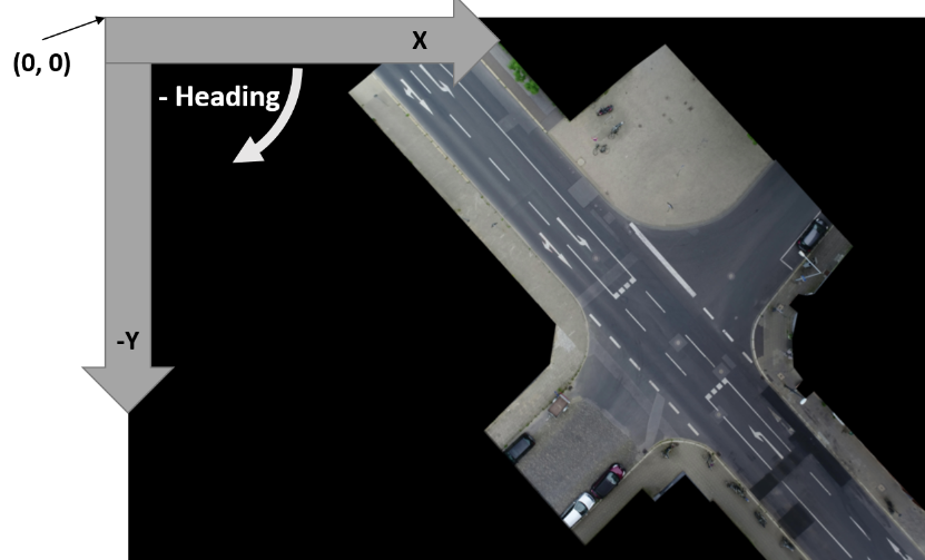
Coordinate System¶

The global coordinate system used is the UTM coordinate system, as we geo-referenced our data. For easier handling of data of the same intersection in different recordings, we introduced a local UTM-like coordinate system.

The only difference is, that the origin (0, 0) is very close to the recorded road section and the same for all recordings at each location.

To transform positions into the global UTM coordinate system, just add xUtmOrigin and yUtmOrigin to all positions.

The local coordinate system looks as follows: The horizontal axis is the x-axis, which grows to the right.

The vertical axis is the y-axis, which grows upwards.

The heading is calcuated as in the UTM coordinate system.

Finally, we use SI units only.