highD (LevelX)¶

About¶

The highD dataset was created and published by a team from the Institute for Automotive Engineering (ika) of RWTH Aachen University to promote research in many different domains of mobility. The dataset can therefore be downloaded and used free of charge for academic and research purposes.

This dataset includes post-processed trajectories of 110,500 vehicles including cars and trucks extracted from drone video recordings at German highways around Cologne during 2017 and 2018. At six different locations, 60 recordings were made with an average length of 17 minutes (16.5 h in total) covering a road segment of about 420 m length. Each vehicle is visible for a median duration of 13.6 s.

How to Apply Dataset¶

The highD dataset is free for non-commercial use only. According to the license and protocols, as a third-party, we cannot share any form of this dataset online. Please visit the official website of highD, fill in the application form and send your request.

How to Obtain Map¶

The maps of highD dataset are manually created by Tactics2D, in the format of OpenStreetMap (OSM), labeled in Lanelet2 style. The maps are stored in data/highD_map. You can download them from here

Citation¶

@inproceedings{highD,
    title={The highD Dataset: A Drone Dataset of Naturalistic Vehicle Trajectories on German Highways for Validation of Highly Automated Driving Systems},
    author={Krajewski, Robert and Bock, Julian and Kloeker, Laurent and Eckstein, Lutz},
    booktitle={2018 21st International Conference on Intelligent Transportation Systems (ITSC)},
    pages={2118-2125},
    year={2018},
    doi={10.1109/ITSC.2018.8569552}
}

Data Analysis¶

This part is independently conducted by Tactics2D.

According to meta records:

• Trajectory data files 01-03 are recorded in location 2 (denoted as highD_2)
• Trajectory data files 04-06 are recorded in location 3 (denoted as highD_3)
• Trajectory data files 07-10 are recorded in location 4 (denoted as highD_4)
• Trajectory data files 11-14, 25-57 are recorded in location 1 (denoted as highD_1)
• Trajectory data files 15-24 are recorded in location 5 (denoted as highD_5)
• Trajectory data files 58-60 are recorded in location 6 (denoted as highD_6)

In [1]:

hide_input

%matplotlib inline
import warnings

warnings.filterwarnings("ignore")

import logging

logging.basicConfig(level=logging.WARNING)

import pandas as pd
import polars as pl
import numpy as np
import matplotlib as mpl
import matplotlib.pyplot as plt
import seaborn as sns

%matplotlib inline import warnings warnings.filterwarnings("ignore") import logging logging.basicConfig(level=logging.WARNING) import pandas as pd import polars as pl import numpy as np import matplotlib as mpl import matplotlib.pyplot as plt import seaborn as sns

In [2]:

hide_input

# Setting up parameters for matplotlib
mpl.rcParams.update(
    {
        "figure.dpi": 300,  # 200 for high quality
        "font.family": "DejaVu Sans Mono",
        "font.size": 6,
        "font.stretch": "semi-expanded",
        "animation.html": "jshtml",
        "animation.embed_limit": 5000,
        "axes.edgecolor": "black",
        "axes.linewidth": 0.8,
        "axes.grid": True,
        "grid.color": "#cccccc",
        "axes.facecolor": "white",
    }
)
sns.set_palette("Set2")

# Setting up parameters for matplotlib mpl.rcParams.update( { "figure.dpi": 300, # 200 for high quality "font.family": "DejaVu Sans Mono", "font.size": 6, "font.stretch": "semi-expanded", "animation.html": "jshtml", "animation.embed_limit": 5000, "axes.edgecolor": "black", "axes.linewidth": 0.8, "axes.grid": True, "grid.color": "#cccccc", "axes.facecolor": "white", } ) sns.set_palette("Set2")

In [3]:

hide_input

locations = dict()
dfs_meta = pd.DataFrame()
for i in range(1, 61):
    df_meta = pd.read_csv("../../data/highD/data/%02d_recordingMeta.csv" % i)
    locations[i] = df_meta["locationId"][0]
    dfs_meta = pd.concat([dfs_meta, df_meta], ignore_index=True)

locations = dict() dfs_meta = pd.DataFrame() for i in range(1, 61): df_meta = pd.read_csv("../../data/highD/data/%02d_recordingMeta.csv" % i) locations[i] = df_meta["locationId"][0] dfs_meta = pd.concat([dfs_meta, df_meta], ignore_index=True)

In [4]:

hide_input

dfs_track_meta = pd.DataFrame()
for i in range(1, 61):
    df_track_meta = pd.read_csv("../../data/highD/data/%02d_tracksMeta.csv" % i)
    df_track_meta["locationId"] = locations[i]
    df_track_meta["fileId"] = i
    dfs_track_meta = pd.concat([dfs_track_meta, df_track_meta], ignore_index=True)

dfs_track_meta = pd.DataFrame() for i in range(1, 61): df_track_meta = pd.read_csv("../../data/highD/data/%02d_tracksMeta.csv" % i) df_track_meta["locationId"] = locations[i] df_track_meta["fileId"] = i dfs_track_meta = pd.concat([dfs_track_meta, df_track_meta], ignore_index=True)

Distribution of Trajectory Categories¶

There are two types of vehicles in the highD dataset: Car and Truck. The composition of vehicle types varies significantly across locations, and within each location, the proportion of each vehicle type exhibits noticeable variance. Nevertheless, Car consistently accounts for over 70% of all vehicles, regardless of location.

In [5]:

hide_input

dfs_meta["car_ratio"] = dfs_meta["numCars"] / dfs_meta["numVehicles"]
dfs_meta["locationId"] = pd.Categorical(
    dfs_meta["locationId"], categories=[1, 2, 3, 4, 5, 6], ordered=True
)

dfs_meta["car_ratio"] = dfs_meta["numCars"] / dfs_meta["numVehicles"] dfs_meta["locationId"] = pd.Categorical( dfs_meta["locationId"], categories=[1, 2, 3, 4, 5, 6], ordered=True )

In [6]:

hide_input

f, ax = plt.subplots(figsize=(6, 3))

sns.boxplot(data=dfs_meta, x="car_ratio", y="locationId", width=0.5, ax=ax)

sns.stripplot(data=dfs_meta, x="car_ratio", y="locationId", alpha=0.6, ax=ax)

ax.set_xticks([0.7, 0.8, 0.9, 1.0])
ax.set_xticklabels(["70", "80", "90", "100"])
ax.yaxis.grid(True)
ax.set_xlabel("Proportion of `Car` in each file (%)")
ax.set_ylabel("Location")
plt.show()

f, ax = plt.subplots(figsize=(6, 3)) sns.boxplot(data=dfs_meta, x="car_ratio", y="locationId", width=0.5, ax=ax) sns.stripplot(data=dfs_meta, x="car_ratio", y="locationId", alpha=0.6, ax=ax) ax.set_xticks([0.7, 0.8, 0.9, 1.0]) ax.set_xticklabels(["70", "80", "90", "100"]) ax.yaxis.grid(True) ax.set_xlabel("Proportion of `Car` in each file (%)") ax.set_ylabel("Location") plt.show()

Distribution of X-Velocity¶

X-Velocity refers to the vehicles' speed along the direction of the route. In this visualization, we present the distribution of the minimum, mean, and maximum X-Velocity for each trajectory, grouped by location. Despite being recorded on a highway, the X-Velocity varies significantly among individual drivers. Notably, the distribution shows multiple peaks: one around 23 m/s (approximately 80 km/h), and another around 33 m/s (approximately 120 km/h). However, without accurate mapping to real-world time, it is difficult to determine whether these peaks are caused by rush hour traffic patterns or simply reflect natural differences in driving behavior.

In [7]:

hide_input

dfs_track_meta_melt_by_velocity = dfs_track_meta.melt(
    id_vars="locationId",
    value_vars=["minXVelocity", "maxXVelocity", "meanXVelocity"],
    var_name="XVelocity",
)

dfs_track_meta_melt_by_velocity["locationId"] = pd.Categorical(
    dfs_track_meta_melt_by_velocity["locationId"], categories=[1, 2, 3, 4, 5, 6], ordered=True
)

dfs_track_meta_melt_by_velocity = dfs_track_meta.melt( id_vars="locationId", value_vars=["minXVelocity", "maxXVelocity", "meanXVelocity"], var_name="XVelocity", ) dfs_track_meta_melt_by_velocity["locationId"] = pd.Categorical( dfs_track_meta_melt_by_velocity["locationId"], categories=[1, 2, 3, 4, 5, 6], ordered=True )

In [8]:

hide_input

f, ax = plt.subplots(figsize=(6, 6))
sns.stripplot(
    data=dfs_track_meta_melt_by_velocity,
    x="value",
    y="locationId",
    hue="XVelocity",
    dodge=True,
    alpha=0.15,
    zorder=1,
    jitter=True,
    size=1,
    palette="Set2",
    ax=ax,
)

sns.move_legend(
    ax, loc="upper center", bbox_to_anchor=(0.5, 1.1), ncol=3, markerscale=5, title=None
)

legend = ax.get_legend()
for handle in legend.get_lines():
    handle.set_alpha(1)

ax.set_xlim(0, 70)
ax.set_xticks([0, 10, 20, 30, 40, 50, 60, 70])
ax.set_xticklabels(["0", "10", "20", "30", "40", "50", "60", "70"])
ax.set_xlabel("XVelocity (m/s)")
ax.set_ylabel("Location")
plt.show()

f, ax = plt.subplots(figsize=(6, 6)) sns.stripplot( data=dfs_track_meta_melt_by_velocity, x="value", y="locationId", hue="XVelocity", dodge=True, alpha=0.15, zorder=1, jitter=True, size=1, palette="Set2", ax=ax, ) sns.move_legend( ax, loc="upper center", bbox_to_anchor=(0.5, 1.1), ncol=3, markerscale=5, title=None ) legend = ax.get_legend() for handle in legend.get_lines(): handle.set_alpha(1) ax.set_xlim(0, 70) ax.set_xticks([0, 10, 20, 30, 40, 50, 60, 70]) ax.set_xticklabels(["0", "10", "20", "30", "40", "50", "60", "70"]) ax.set_xlabel("XVelocity (m/s)") ax.set_ylabel("Location") plt.show()

In [9]:

hide_input

dfs = [pl.DataFrame()] * 6

for i in range(1, 61):
    df = pl.read_csv("../../data/highD/data/%02d_tracks.csv" % i)
    df = df.select(["id", "frame", "x", "y", "xVelocity", "yVelocity", "laneId"])
    df = df.with_columns(pl.lit(i).alias("fileId"))
    df = df.join(
        pl.DataFrame(dfs_track_meta)[["fileId", "id", "class"]], on=["fileId", "id"], how="left"
    )

    dfs[locations[i] - 1] = pl.concat([dfs[locations[i] - 1], df])

dfs = [pl.DataFrame()] * 6 for i in range(1, 61): df = pl.read_csv("../../data/highD/data/%02d_tracks.csv" % i) df = df.select(["id", "frame", "x", "y", "xVelocity", "yVelocity", "laneId"]) df = df.with_columns(pl.lit(i).alias("fileId")) df = df.join( pl.DataFrame(dfs_track_meta)[["fileId", "id", "class"]], on=["fileId", "id"], how="left" ) dfs[locations[i] - 1] = pl.concat([dfs[locations[i] - 1], df])

In [10]:

hide_input

for i in range(6):
    x_min = np.floor(dfs[i]["x"].min())
    x_max = np.ceil(dfs[i]["x"].max())
    y_min = np.floor(dfs[i]["y"].min())
    y_max = np.ceil(dfs[i]["y"].max())
    vx = dfs[i]["xVelocity"].to_numpy()
    vy = dfs[i]["yVelocity"].to_numpy()

    x_edges_1 = np.linspace(x_min, x_max, num=int((x_max - x_min) * 10 + 1), endpoint=True)
    y_edges_1 = np.linspace(y_min, y_max, num=int((y_max - y_min) * 10 + 1), endpoint=True)
    x_bin_1 = np.digitize(dfs[i]["x"].to_numpy(), x_edges_1) - 1
    y_bin_1 = np.digitize(dfs[i]["y"].to_numpy(), y_edges_1) - 1
    x_edges_2 = np.linspace(x_min, x_max, num=int((x_max - x_min) * 2 + 1), endpoint=True)
    y_edges_2 = np.linspace(y_min, y_max, num=int((y_max - y_min) * 2 + 1), endpoint=True)
    x_bin_2 = np.digitize(dfs[i]["x"].to_numpy(), x_edges_2) - 1
    y_bin_2 = np.digitize(dfs[i]["y"].to_numpy(), y_edges_2) - 1
    speed = np.sqrt(vx**2 + vy**2)
    heading = np.arctan(vy / vx)

    dfs[i] = dfs[i].with_columns(
        [
            pl.Series("x_bin_1", x_bin_1),
            pl.Series("y_bin_1", y_bin_1),
            pl.Series("x_bin_2", x_bin_2),
            pl.Series("y_bin_2", y_bin_2),
            pl.Series("speed (m/s)", speed),
            pl.Series("heading (radian)", heading),
        ]
    )

for i in range(6): x_min = np.floor(dfs[i]["x"].min()) x_max = np.ceil(dfs[i]["x"].max()) y_min = np.floor(dfs[i]["y"].min()) y_max = np.ceil(dfs[i]["y"].max()) vx = dfs[i]["xVelocity"].to_numpy() vy = dfs[i]["yVelocity"].to_numpy() x_edges_1 = np.linspace(x_min, x_max, num=int((x_max - x_min) * 10 + 1), endpoint=True) y_edges_1 = np.linspace(y_min, y_max, num=int((y_max - y_min) * 10 + 1), endpoint=True) x_bin_1 = np.digitize(dfs[i]["x"].to_numpy(), x_edges_1) - 1 y_bin_1 = np.digitize(dfs[i]["y"].to_numpy(), y_edges_1) - 1 x_edges_2 = np.linspace(x_min, x_max, num=int((x_max - x_min) * 2 + 1), endpoint=True) y_edges_2 = np.linspace(y_min, y_max, num=int((y_max - y_min) * 2 + 1), endpoint=True) x_bin_2 = np.digitize(dfs[i]["x"].to_numpy(), x_edges_2) - 1 y_bin_2 = np.digitize(dfs[i]["y"].to_numpy(), y_edges_2) - 1 speed = np.sqrt(vx**2 + vy**2) heading = np.arctan(vy / vx) dfs[i] = dfs[i].with_columns( [ pl.Series("x_bin_1", x_bin_1), pl.Series("y_bin_1", y_bin_1), pl.Series("x_bin_2", x_bin_2), pl.Series("y_bin_2", y_bin_2), pl.Series("speed (m/s)", speed), pl.Series("heading (radian)", heading), ] )

Distribution of Average Speed on Map¶

We present a heatmap of the average vehicle speed at each location. The tight clustering of data points suggests that vehicle positions have already been calibrated, and the variation across different files is negligible.

Notably, vehicles in the outer (leftmost) lanes tend to have lower average speeds compared to those in the inner (rightmost) lanes, which aligns with common traffic patterns. The average speed at some lanes exceeds 50 m/s (180 km/h), highlighting a distinctive feature of German highways, where no speed limit is enforced on certain sections.

In [11]:

hide_input

fig, axes = plt.subplots(6, 1, figsize=(6, 3), sharex=True, sharey=True)

for i in range(6):
    df_speed_heatmap = (
        dfs[i]
        .group_by(["y_bin_1", "x_bin_1"])
        .agg(pl.col("speed (m/s)").mean().alias("avg_speed"))
        .sort(["y_bin_1", "x_bin_1"])
    ).to_pandas()
    grid = df_speed_heatmap.pivot(index="y_bin_1", columns="x_bin_1", values="avg_speed")
    hm = sns.heatmap(
        grid,
        ax=axes[i],
        cmap="cool",
        cbar=False,
        xticklabels=False,
        yticklabels=False,
        vmin=0,
        vmax=70,
    )

    for spine in axes[i].spines.values():
        spine.set_visible(True)
        spine.set_color("gray")
        spine.set_linewidth(0.5)
    axes[i].set_aspect("equal")
    axes[i].set_xlabel("")
    axes[i].set_ylabel(f"{i+1}", rotation=0)

cbar_ax = fig.add_axes([0.1, 0.94, 0.8, 0.02])
cbar = fig.colorbar(hm.get_children()[0], cax=cbar_ax, orientation="horizontal")
fig.text(0.02, 0.5, "Location", va="center", rotation="vertical")

plt.tight_layout(rect=[0.04, 0, 1, 0.9])
plt.show()

fig, axes = plt.subplots(6, 1, figsize=(6, 3), sharex=True, sharey=True) for i in range(6): df_speed_heatmap = ( dfs[i] .group_by(["y_bin_1", "x_bin_1"]) .agg(pl.col("speed (m/s)").mean().alias("avg_speed")) .sort(["y_bin_1", "x_bin_1"]) ).to_pandas() grid = df_speed_heatmap.pivot(index="y_bin_1", columns="x_bin_1", values="avg_speed") hm = sns.heatmap( grid, ax=axes[i], cmap="cool", cbar=False, xticklabels=False, yticklabels=False, vmin=0, vmax=70, ) for spine in axes[i].spines.values(): spine.set_visible(True) spine.set_color("gray") spine.set_linewidth(0.5) axes[i].set_aspect("equal") axes[i].set_xlabel("") axes[i].set_ylabel(f"{i+1}", rotation=0) cbar_ax = fig.add_axes([0.1, 0.94, 0.8, 0.02]) cbar = fig.colorbar(hm.get_children()[0], cax=cbar_ax, orientation="horizontal") fig.text(0.02, 0.5, "Location", va="center", rotation="vertical") plt.tight_layout(rect=[0.04, 0, 1, 0.9]) plt.show()

Distribution of Lane Change Frequency on Map¶

The figure illustrates the cumulative count of lane-changing events within each predefined grid cell on the map. Lane changing events happen sporadically along the lanes, without showing a strong spatial pattern. This is likely because the data was collected on relatively stable highway segments, where vehicles generally follow consistent driving behavior and lane usage is less influenced by external factors such as intersections or merges.

In [12]:

hide_input

fig, axes = plt.subplots(6, 1, figsize=(6, 3), sharex=True, sharey=True)

for i in range(6):
    df_lane_changing = dfs[i].to_pandas()
    df_lane_changing = df_lane_changing.sort_values(by=["fileId", "id", "frame"])
    df_lane_changing["prev_laneId"] = df_lane_changing.groupby(["fileId", "id"])["laneId"].shift(1)
    df_lane_changing["laneChange"] = (
        df_lane_changing["laneId"] != df_lane_changing["prev_laneId"]
    ).astype(int)
    first_row_mask = df_lane_changing.groupby(["fileId", "id"]).cumcount() == 0
    df_lane_changing.loc[first_row_mask, "laneChange"] = 0
    df_lane_changing_heatmap = (
        df_lane_changing.groupby(["y_bin_2", "x_bin_2"])["laneChange"].sum().unstack(fill_value=0)
    )
    mask = df_lane_changing_heatmap == 0
    hm = sns.heatmap(
        df_lane_changing_heatmap,
        mask=mask,
        ax=axes[i],
        cmap="cool",
        cbar=False,
        xticklabels=False,
        yticklabels=False,
        vmin=0,
        vmax=3,
    )

    for spine in axes[i].spines.values():
        spine.set_visible(True)
        spine.set_color("gray")
        spine.set_linewidth(0.5)
    axes[i].set_aspect("equal")
    axes[i].set_xlabel("")
    axes[i].set_ylabel(f"{i+1}", rotation=0)

cbar_ax = fig.add_axes([0.1, 0.94, 0.8, 0.02])
cbar = fig.colorbar(hm.get_children()[0], cax=cbar_ax, orientation="horizontal")
fig.text(0.02, 0.5, "Location", va="center", rotation="vertical")

plt.tight_layout(rect=[0.04, 0, 1, 0.9])
plt.show()

fig, axes = plt.subplots(6, 1, figsize=(6, 3), sharex=True, sharey=True) for i in range(6): df_lane_changing = dfs[i].to_pandas() df_lane_changing = df_lane_changing.sort_values(by=["fileId", "id", "frame"]) df_lane_changing["prev_laneId"] = df_lane_changing.groupby(["fileId", "id"])["laneId"].shift(1) df_lane_changing["laneChange"] = ( df_lane_changing["laneId"] != df_lane_changing["prev_laneId"] ).astype(int) first_row_mask = df_lane_changing.groupby(["fileId", "id"]).cumcount() == 0 df_lane_changing.loc[first_row_mask, "laneChange"] = 0 df_lane_changing_heatmap = ( df_lane_changing.groupby(["y_bin_2", "x_bin_2"])["laneChange"].sum().unstack(fill_value=0) ) mask = df_lane_changing_heatmap == 0 hm = sns.heatmap( df_lane_changing_heatmap, mask=mask, ax=axes[i], cmap="cool", cbar=False, xticklabels=False, yticklabels=False, vmin=0, vmax=3, ) for spine in axes[i].spines.values(): spine.set_visible(True) spine.set_color("gray") spine.set_linewidth(0.5) axes[i].set_aspect("equal") axes[i].set_xlabel("") axes[i].set_ylabel(f"{i+1}", rotation=0) cbar_ax = fig.add_axes([0.1, 0.94, 0.8, 0.02]) cbar = fig.colorbar(hm.get_children()[0], cax=cbar_ax, orientation="horizontal") fig.text(0.02, 0.5, "Location", va="center", rotation="vertical") plt.tight_layout(rect=[0.04, 0, 1, 0.9]) plt.show()

Distribution of Speed by Vehicle Type¶

The speed distribution differs significantly between vehicle types. Vehicles of the same type tend to exhibit similar speed distribution patterns across different locations.

In [13]:

hide_input

fig, axes = plt.subplots(3, 2, figsize=(6, 6), sharex=True)
for i in range(6):
    df_speed = dfs[i].to_pandas()
    sns.histplot(
        df_speed,
        x="speed (m/s)",
        hue="class",
        hue_order=["Car", "Truck"],
        multiple="layer",
        palette="Set2",
        ax=axes[int(i // 2)][int(i % 2)],
        stat="density",
        common_norm=False,
        binwidth=1,
        binrange=(0, 70),
        linewidth=0,
        alpha=0.5,
        legend=(i == 1),
    )

    axes[int(i // 2)][int(i % 2)].set_xlim([0, 70])
    axes[int(i // 2)][int(i % 2)].set_ylabel(f"Location {i+1}")
    axes[int(i // 2)][int(i % 2)].set_ylim([0, 0.4])
    axes[int(i // 2)][int(i % 2)].set_yticks([0, 0.1, 0.2, 0.3, 0.4])

fig.text(0.02, 0.5, "Probability Density", va="center", rotation="vertical")

fig.tight_layout(rect=[0.03, 0, 1, 1])
plt.show()

fig, axes = plt.subplots(3, 2, figsize=(6, 6), sharex=True) for i in range(6): df_speed = dfs[i].to_pandas() sns.histplot( df_speed, x="speed (m/s)", hue="class", hue_order=["Car", "Truck"], multiple="layer", palette="Set2", ax=axes[int(i // 2)][int(i % 2)], stat="density", common_norm=False, binwidth=1, binrange=(0, 70), linewidth=0, alpha=0.5, legend=(i == 1), ) axes[int(i // 2)][int(i % 2)].set_xlim([0, 70]) axes[int(i // 2)][int(i % 2)].set_ylabel(f"Location {i+1}") axes[int(i // 2)][int(i % 2)].set_ylim([0, 0.4]) axes[int(i // 2)][int(i % 2)].set_yticks([0, 0.1, 0.2, 0.3, 0.4]) fig.text(0.02, 0.5, "Probability Density", va="center", rotation="vertical") fig.tight_layout(rect=[0.03, 0, 1, 1]) plt.show()

Distribution of Heading by Vehicle Type¶

We present a relative heading angle with respect to the direction of the route. The heading distribution of different types shows high similarity at each location. Since the scenario takes place on a highway, the heading does not deviate significantly from the route direction, with the jitter mostly kept within 0.02 radians.

In [14]:

hide_input

fig, axes = plt.subplots(3, 2, figsize=(6, 6), sharex=True)
for i in range(6):
    df_heading = dfs[i].to_pandas()
    sns.histplot(
        df_heading,
        x="heading (radian)",
        hue="class",
        hue_order=["Car", "Truck"],
        multiple="layer",
        palette="Set2",
        ax=axes[int(i // 2)][int(i % 2)],
        stat="density",
        common_norm=False,
        binwidth=0.002,
        binrange=(-0.1, 0.1),
        linewidth=0,
        alpha=0.5,
        legend=(i == 1),
    )

    axes[int(i // 2)][int(i % 2)].set_xlim([-0.1, 0.1])
    axes[int(i // 2)][int(i % 2)].set_xticks([-0.1, -0.05, 0, 0.05, 0.1])
    axes[int(i // 2)][int(i % 2)].set_ylim([0, 150])
    axes[int(i // 2)][int(i % 2)].set_yticks([0, 50, 100, 150])
    axes[int(i // 2)][int(i % 2)].set_ylabel(f"Location {i+1}")

fig.text(0.02, 0.5, "Probability Density", va="center", rotation="vertical")

fig.tight_layout(rect=[0.03, 0, 1, 1])
plt.show()

fig, axes = plt.subplots(3, 2, figsize=(6, 6), sharex=True) for i in range(6): df_heading = dfs[i].to_pandas() sns.histplot( df_heading, x="heading (radian)", hue="class", hue_order=["Car", "Truck"], multiple="layer", palette="Set2", ax=axes[int(i // 2)][int(i % 2)], stat="density", common_norm=False, binwidth=0.002, binrange=(-0.1, 0.1), linewidth=0, alpha=0.5, legend=(i == 1), ) axes[int(i // 2)][int(i % 2)].set_xlim([-0.1, 0.1]) axes[int(i // 2)][int(i % 2)].set_xticks([-0.1, -0.05, 0, 0.05, 0.1]) axes[int(i // 2)][int(i % 2)].set_ylim([0, 150]) axes[int(i // 2)][int(i % 2)].set_yticks([0, 50, 100, 150]) axes[int(i // 2)][int(i % 2)].set_ylabel(f"Location {i+1}") fig.text(0.02, 0.5, "Probability Density", va="center", rotation="vertical") fig.tight_layout(rect=[0.03, 0, 1, 1]) plt.show()

Tactics2D Integration¶

This section explains how to parse and replay logs from the highD dataset by Tactics2D.

Dataset Preparation¶

You can place the highD dataset in any directory of your choice. However, it’s important to maintain the following folder structure for compatibility:

highD
├── data
│   ├── 01_highway.png
│   ├── 01_recordingMeta.csv
│   ├── 01_tracks.csv
│   ├── 01_tracksMeta.csv
│   ├── ...

Class Mapping¶

The table below illustrates how classes from the highD dataset are mapped to corresponding traffic participants in the Tactics2D framework. In this mapping, both cars and trucks from highD are represented as the generic Vehicle class within Tactics2D.

highD Class	Tactics2D Class
Car	tactics2d.participant.element.Vehicle
Truck	tactics2d.participant.element.Vehicle

Parse and Replay Logs¶

To parse, replay, and visualize the highD dataset using Tactics2D, you can use the following code snippet:

In [15]:

%matplotlib notebook

import os

import numpy as np
from matplotlib.animation import FuncAnimation
from shapely.geometry import Point
from IPython.display import HTML

from tactics2d.dataset_parser import LevelXParser
from tactics2d.map.parser import OSMParser
from tactics2d.map.map_config import HIGHD_MAP_CONFIG
from tactics2d.sensor import BEVCamera
from tactics2d.renderer import MatplotlibRenderer

%matplotlib notebook import os import numpy as np from matplotlib.animation import FuncAnimation from shapely.geometry import Point from IPython.display import HTML from tactics2d.dataset_parser import LevelXParser from tactics2d.map.parser import OSMParser from tactics2d.map.map_config import HIGHD_MAP_CONFIG from tactics2d.sensor import BEVCamera from tactics2d.renderer import MatplotlibRenderer

Specify the path to the dataset and the map, and then run the following code:

In [16]:

dataset_path = "../../data/highD/data"  # Replace with your dataset path
map_path = "../../data/highD_map"  # Replace with your map path
dataset_parser = LevelXParser("highD")
map_parser = OSMParser(lanelet2=True)

dataset_path = "../../data/highD/data" # Replace with your dataset path map_path = "../../data/highD_map" # Replace with your map path dataset_parser = LevelXParser("highD") map_parser = OSMParser(lanelet2=True)

For simplicity, we revise a function from the ScenarioManager to handle the parsing and replaying of the highD dataset:

In [17]:

def render_levelx(map_, participants, map_boundary, time_range):
    x_min, x_max, y_min, y_max = map_boundary
    camera_position = np.array([0, 0])
    camera = BEVCamera(id_=0, map_=map_)

    renderer = MatplotlibRenderer(
        xlim=(x_min, x_max), ylim=(y_min, y_max), resolution=(1600, 300), auto_scale=False
    )

    fig = renderer.fig  # Use the one already created
    fig.set_dpi(200)
    frame_list = list(range(time_range[0], time_range[1], 40))
    prev_road_id_set = set()
    prev_participant_id_set = set()

    def update(frame):
        nonlocal prev_road_id_set, prev_participant_id_set

        participant_ids = [pid for pid, p in participants.items() if p.is_active(frame)]

        geometry_data, prev_road_id_set, prev_participant_id_set = camera.update(
            frame,
            participants,
            participant_ids,
            prev_road_id_set,
            prev_participant_id_set,
            Point(camera_position),
        )

        renderer.update(geometry_data)
        renderer.ax.set_title(f"Frame: {frame}")

    ani = FuncAnimation(fig, update, frames=frame_list, interval=40, repeat=True)
    return ani

def render_levelx(map_, participants, map_boundary, time_range): x_min, x_max, y_min, y_max = map_boundary camera_position = np.array([0, 0]) camera = BEVCamera(id_=0, map_=map_) renderer = MatplotlibRenderer( xlim=(x_min, x_max), ylim=(y_min, y_max), resolution=(1600, 300), auto_scale=False ) fig = renderer.fig # Use the one already created fig.set_dpi(200) frame_list = list(range(time_range[0], time_range[1], 40)) prev_road_id_set = set() prev_participant_id_set = set() def update(frame): nonlocal prev_road_id_set, prev_participant_id_set participant_ids = [pid for pid, p in participants.items() if p.is_active(frame)] geometry_data, prev_road_id_set, prev_participant_id_set = camera.update( frame, participants, participant_ids, prev_road_id_set, prev_participant_id_set, Point(camera_position), ) renderer.update(geometry_data) renderer.ax.set_title(f"Frame: {frame}") ani = FuncAnimation(fig, update, frames=frame_list, interval=40, repeat=True) return ani

In [18]:

participants, actual_time_range = dataset_parser.parse_trajectory(
    file=11, folder=dataset_path, time_range=(0, 10000)
)
map_ = map_parser.parse(
    file_path=os.path.join(map_path, "highD_1.osm"), configs=HIGHD_MAP_CONFIG["highD_1"]
)

print(f"Map boundary of HighD location 1: {map_.boundary}.")

boundary = (
    map_.boundary[0] + 100,
    map_.boundary[1] - 100,
    map_.boundary[2] - 20,
    map_.boundary[3] + 20,
)

ani = render_levelx(map_, participants, boundary, actual_time_range)
HTML(ani.to_html5_video())

participants, actual_time_range = dataset_parser.parse_trajectory( file=11, folder=dataset_path, time_range=(0, 10000) ) map_ = map_parser.parse( file_path=os.path.join(map_path, "highD_1.osm"), configs=HIGHD_MAP_CONFIG["highD_1"] ) print(f"Map boundary of HighD location 1: {map_.boundary}.") boundary = ( map_.boundary[0] + 100, map_.boundary[1] - 100, map_.boundary[2] - 20, map_.boundary[3] + 20, ) ani = render_levelx(map_, participants, boundary, actual_time_range) HTML(ani.to_html5_video())

Map boundary of HighD location 1: (np.float64(-112.0), np.float64(558.0), np.float64(-29.0), np.float64(0.0)).

Out[18]:

In the same way, we display the log in other locations in highD.

In [19]:

hide_input

participants, actual_time_range = dataset_parser.parse_trajectory(
    file=1, folder=dataset_path, time_range=(10000, 20000)
)
map_ = map_parser.parse(
    file_path=os.path.join(map_path, "highD_2.osm"), configs=HIGHD_MAP_CONFIG["highD_2"]
)

print(f"Map boundary of HighD location 2: {map_.boundary}.")

boundary = (
    map_.boundary[0] + 100,
    map_.boundary[1] - 100,
    map_.boundary[2] - 20,
    map_.boundary[3] + 20,
)

ani = render_levelx(map_, participants, boundary, actual_time_range)
HTML(ani.to_html5_video())

participants, actual_time_range = dataset_parser.parse_trajectory( file=1, folder=dataset_path, time_range=(10000, 20000) ) map_ = map_parser.parse( file_path=os.path.join(map_path, "highD_2.osm"), configs=HIGHD_MAP_CONFIG["highD_2"] ) print(f"Map boundary of HighD location 2: {map_.boundary}.") boundary = ( map_.boundary[0] + 100, map_.boundary[1] - 100, map_.boundary[2] - 20, map_.boundary[3] + 20, ) ani = render_levelx(map_, participants, boundary, actual_time_range) HTML(ani.to_html5_video())

Map boundary of HighD location 2: (np.float64(-112.0), np.float64(558.0), np.float64(-21.0), np.float64(0.0)).

Out[19]:

In [20]:

hide_input

participants, actual_time_range = dataset_parser.parse_trajectory(
    file=4, folder=dataset_path, time_range=(20000, 30000)
)
map_ = map_parser.parse(
    file_path=os.path.join(map_path, "highD_3.osm"), configs=HIGHD_MAP_CONFIG["highD_3"]
)

print(f"Map boundary of HighD location 3: {map_.boundary}.")

boundary = (
    map_.boundary[0] + 100,
    map_.boundary[1] - 100,
    map_.boundary[2] - 20,
    map_.boundary[3] + 20,
)

ani = render_levelx(map_, participants, boundary, actual_time_range)
HTML(ani.to_html5_video())

participants, actual_time_range = dataset_parser.parse_trajectory( file=4, folder=dataset_path, time_range=(20000, 30000) ) map_ = map_parser.parse( file_path=os.path.join(map_path, "highD_3.osm"), configs=HIGHD_MAP_CONFIG["highD_3"] ) print(f"Map boundary of HighD location 3: {map_.boundary}.") boundary = ( map_.boundary[0] + 100, map_.boundary[1] - 100, map_.boundary[2] - 20, map_.boundary[3] + 20, ) ani = render_levelx(map_, participants, boundary, actual_time_range) HTML(ani.to_html5_video())

Map boundary of HighD location 3: (np.float64(-112.0), np.float64(558.0), np.float64(-25.0), np.float64(0.0)).

Out[20]:

In [21]:

hide_input

participants, actual_time_range = dataset_parser.parse_trajectory(
    file=7, folder=dataset_path, time_range=(30000, 40000)
)
map_ = map_parser.parse(
    file_path=os.path.join(map_path, "highD_4.osm"), configs=HIGHD_MAP_CONFIG["highD_4"]
)

print(f"Map boundary of HighD location 4: {map_.boundary}.")

boundary = (
    map_.boundary[0] + 100,
    map_.boundary[1] - 100,
    map_.boundary[2] - 20,
    map_.boundary[3] + 20,
)

ani = render_levelx(map_, participants, boundary, actual_time_range)
HTML(ani.to_html5_video())

participants, actual_time_range = dataset_parser.parse_trajectory( file=7, folder=dataset_path, time_range=(30000, 40000) ) map_ = map_parser.parse( file_path=os.path.join(map_path, "highD_4.osm"), configs=HIGHD_MAP_CONFIG["highD_4"] ) print(f"Map boundary of HighD location 4: {map_.boundary}.") boundary = ( map_.boundary[0] + 100, map_.boundary[1] - 100, map_.boundary[2] - 20, map_.boundary[3] + 20, ) ani = render_levelx(map_, participants, boundary, actual_time_range) HTML(ani.to_html5_video())

Map boundary of HighD location 4: (np.float64(-112.0), np.float64(558.0), np.float64(-27.0), np.float64(0.0)).

Out[21]:

In [22]:

hide_input

participants, actual_time_range = dataset_parser.parse_trajectory(
    file=15, folder=dataset_path, time_range=(40000, 50000)
)
map_ = map_parser.parse(
    file_path=os.path.join(map_path, "highD_5.osm"), configs=HIGHD_MAP_CONFIG["highD_5"]
)

print(f"Map boundary of HighD location 5: {map_.boundary}.")

boundary = (
    map_.boundary[0] + 100,
    map_.boundary[1] - 100,
    map_.boundary[2] - 20,
    map_.boundary[3] + 20,
)

ani = render_levelx(map_, participants, boundary, actual_time_range)
HTML(ani.to_html5_video())

participants, actual_time_range = dataset_parser.parse_trajectory( file=15, folder=dataset_path, time_range=(40000, 50000) ) map_ = map_parser.parse( file_path=os.path.join(map_path, "highD_5.osm"), configs=HIGHD_MAP_CONFIG["highD_5"] ) print(f"Map boundary of HighD location 5: {map_.boundary}.") boundary = ( map_.boundary[0] + 100, map_.boundary[1] - 100, map_.boundary[2] - 20, map_.boundary[3] + 20, ) ani = render_levelx(map_, participants, boundary, actual_time_range) HTML(ani.to_html5_video())

Map boundary of HighD location 5: (np.float64(-112.0), np.float64(558.0), np.float64(-21.0), np.float64(0.0)).

Out[22]:

In [23]:

hide_input

participants, actual_time_range = dataset_parser.parse_trajectory(
    file=58, folder=dataset_path, time_range=(50000, 60000)
)
map_ = map_parser.parse(
    file_path=os.path.join(map_path, "highD_6.osm"), configs=HIGHD_MAP_CONFIG["highD_6"]
)

print(f"Map boundary of HighD location 6: {map_.boundary}.")

boundary = (
    map_.boundary[0] + 100,
    map_.boundary[1] - 100,
    map_.boundary[2] - 20,
    map_.boundary[3] + 20,
)

ani = render_levelx(map_, participants, boundary, actual_time_range)
HTML(ani.to_html5_video())

participants, actual_time_range = dataset_parser.parse_trajectory( file=58, folder=dataset_path, time_range=(50000, 60000) ) map_ = map_parser.parse( file_path=os.path.join(map_path, "highD_6.osm"), configs=HIGHD_MAP_CONFIG["highD_6"] ) print(f"Map boundary of HighD location 6: {map_.boundary}.") boundary = ( map_.boundary[0] + 100, map_.boundary[1] - 100, map_.boundary[2] - 20, map_.boundary[3] + 20, ) ani = render_levelx(map_, participants, boundary, actual_time_range) HTML(ani.to_html5_video())

Map boundary of HighD location 6: (np.float64(-112.0), np.float64(558.0), np.float64(-27.0), np.float64(4.0)).

Out[23]:

Appendix: Data Format¶

Note

This is a backup copy of the official documentation , provided here for reference purposes only.

The highD dataset includes data extracted from 60 recordings. For each recording, in total four files are provided:

• An image of the recorded highway section (XX_highway.jpg)
• A csv file describing the recording location (XX_recordingMeta.csv)
• A csv file containing an overview of recorded vehicle tracks (XX_tracksMeta.csv)
• A csv file for the tracks' trajectories. These files are created for each recording to ensure easy handling of the data. In the following, the dataset format and especially the meaning of every column is explained in detail. (XX_tracks.csv)

Image of the Highway Section¶

For each recording an image of the highway section is added. The image was created from the used recording itself by removing all vehicles through a filter. Additionally the resolution of the image was reduced.

Recording Meta Information¶

This file contains metadata for each recording. The metadata provides a general overview, e.g. of the time of recording, the highway section considered and the total number of vehicles recorded.

Name	Description	Unit
id	The id of the recording. Every recording has a unique id.	[-]
frameRate	The frame rate which was used to record the video.	[hz]
locationId	The id of the recording location. In total six different locations exist in the dataset.	[-]
speedLimit	The speed limit of the driving lanes. In all recordings, the speed limit is the same for every driving lane.	[m/s]
month	The month the recording was done.	[-]
weekDay	The week day the recording was done.	[-]
startTime	The start time at which the recording was done.	[hh:mm]
duration	The duration of the recording.	[s]
totalDrivenDistance	The total driven distance of all tracked vehicles.	[m]
totalDrivenTime	The total driven time of all tracked vehicles.	[s]
numVehicles	The number of vehicles tracked including cars and trucks.	[-]
numCars	The number of cars tracked.	[-]
numTrucks	The number of trucks tracked.	[-]
upperLaneMarkings	The y positions of the upper lane markings. The positions are separated by a ";".	[m]
lowerLaneMarkings	The y positions of the lower lane markings. The positions are separated by a ";".	[m]

Track Meta Information¶

This file contains an overview of all tracks. For each track there are summary values like the distance covered or the average speed. The purpose of this file is to allow to filter tracks e.g. by class or driving direction.

Name	Description	Unit
id	The id of the track. The ids are assigned in ascending order.	[-]
width	The width of the post-processed bounding box of the vehicle. This corresponds to the length of the vehicle.	[m]
height	The height of the post-processed bounding box of the vehicle. This corresponds to the width of the vehicle.	[m]
initialFrame	The initial frame in which the vehicle track starts.	[-]
finalFrame	The frame in which the track of the vehicle ends.	[-]
numFrames	The total lifetime of the track as number of frames.	[-]
class	The vehicle class of the tracked vehicle (Car or Truck).	[-]
drivingDirection	The driving direction of the vehicle. Either 1 for the left direction (upper lanes) or 2 for the right direction (lower lanes).	[-]
traveledDistance	The distance covered by the track.	[m]
minXVelocity	The minimal velocity in driving direction.	[m/s]
maxXVelocity	The maximal velocity in driving direction.	[m/s]
meanXVelocity	The mean velocity in driving direction.	[m/s]
minDHW	The minimal Distance Headway (DHW). This value is set to -1, if no preceding vehicle exists.	[m]
minTHW	The minimal Time Headway (THW). This value is set to -1, if no preceding vehicle exists.	[s]
minTTC	The minimal Time-to-Collision (TTC). This value is set to -1, if no preceding vehicle or valid TTC exists.	[s]
numLaneChanges	Number of lane changes detected by changing lane id.	[-]

Tracks¶

This file contains all time dependent values for each track. Information such as current velocities, viewing ranges and information about surrounding vehicles are included.

Name	Description	Unit
frame	The current frame.	[-]
id	The track's id.	[-]
x	The x position of the upper left corner of the vehicle's bounding box.	[m]
y	The y position of the upper left corner of the vehicle's bounding box.	[m]
width	The width of the bounding box of the vehicle.	[m]
height	The height of the bounding box of the vehicle.	[m]
xVelocity	The longitudinal velocity in the image coordinate system.	[m/s]
yVelocity	The lateral velocity in the image coordinate system.	[m/s]
xAcceleration	The longitudinal acceleration in the image coordinate system.	[m/s²]
yAcceleration	The lateral acceleration in the image coordinate system	[m/s²]
frontSightDistance	The distance to the end of the recorded highway section in driving direction from the vehicle's center.	[m]
backSightDistance	The distance to the end of the recorded highway section in the opposite driving direction from the vehicle's center.	[m]
dhw	The Distance Headway. This value is set to 0, if no preceding vehicle exists.	[m]
thw	The Time Headway. This value is set to 0, if no preceding vehicle exists.	[s]
ttc	The Time-to-Collision. This value is set to 0, if no preceding vehicle or valid TTC exists.	[s]
precedingXVelocity	The longitudinal velocity of the preceding in the image coordinate system. This value is set to 0, if no preceding vehicle exists.	[-]
precedingId	The id of the preceding vehicle in the same lane. This value is set to 0, if no preceding vehicle exists.	[-]
followingId	The id of the following vehicle in the same lane. This value is set to 0, if no following vehicle exists.	[-]
leftPrecedingId	The id of the preceding vehicle on the adjacent lane on the left in the direction of travel. This value is set to 0, if no such a vehicle exists.	[-]
leftAlongsideId	The id of the adjacent vehicle on the adjacent lane on the left in the direction of travel. In order for a vehicle to be adjacent and not e.g. preceding, the vehicles must overlap in the longitudinal direction. This value is set to 0, if no such a vehicle exists.	[-]
leftFollowingId	The id of the following vehicle on the adjacent lane on the left in the direction of travel. This value is set to 0, if no such a vehicle exists.	[-]
rightPrecedingId	The id of the preceding vehicle on the adjacent lane on the right in the direction of travel. This value is set to 0, if no such a vehicle exists.	[-]
rightAlsongsideId	The id of the adjacent vehicle on the adjacent lane on the right in the direction of travel. In order for a vehicle to be adjacent and not e.g. preceding, the vehicles must overlap in the longitudinal direction. This value is set to 0, if no such a vehicle exists.	[-]
rightFollowingId	The id of the following vehicle on the adjacent lane on the right in the direction of travel. This value is set to 0, if no such a vehicle exists.	[-]
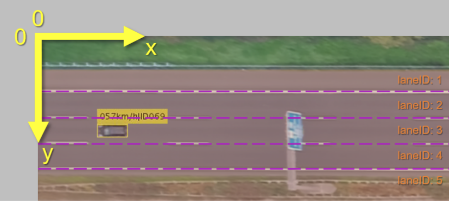
laneId	The IDs start at 1 and are assigned in ascending order. Since the Lane ids are derived from the positions of the lane markings, the first and last ids typically do not describe any useable lanes. For details, see the definition of the coordinate system.	[-]

Coordinate System¶

The global coordinate system used corresponds to the image coordinate system of the video recording. This means that the origin of the coordinate system is in the upper left corner, as shown in the image. The horizontal axis is the x-axis. This corresponds to the direction of travel of the vehicles and grows to the right. The vertical axis is the y-axis. However, this axis grows downwards. In addition no units in pixels are used, since all sizes were converted into SI units. The video recordings were stabilized so that the lane markings run horizontally in the image. Therefore, their positions can be indicated by a y-coordinate. The individual lanes were numbered starting with 1. The areas above the uppermost lane mark, between the driving directions and below the lowermost lane mark are also taken into account for counting. All data is given in the global coordinate system unless otherwise specified. This means that a vehicle on the upper lanes in the image is moving to the left and therefore has a negative speed in X direction.