exiD (LevelX)¶

About¶

The exiD dataset was created and published by a team from the Institute for Automotive Engineering (ika) of RWTH Aachen University to promote research in many different domains of mobility. The dataset can therefore be downloaded and used free of charge for academic and research purposes.

This dataset contains 92 separate recordings (more than 16 hours of video) with traffic at seven different measurement locations at entries and exits of the German Autobahn...The data also contains variations in form of different speed limits on the highways: four locations have no speed limit, two locations have a speed limit of 100 km/h and one location has a speed limit of 120 km/h.

How to Apply¶

The exiD dataset is free for non-commercial use only. According to the license and protocols, as a third-party, we cannot share any form of this dataset online. Please visit the official website of exiD, fill in the application form and send your request.

Citation¶

@inproceedings{exiD,
    title={The exiD Dataset: A Real-World Trajectory Dataset of Highly Interactive Highway Scenarios in Germany},
    author={Moers, Tobias and Vater, Lennart and Krajewski, Robert and Bock, Julian and Zlocki, Adrian and Eckstein, Lutz},
    booktitle={2022 IEEE Intelligent Vehicles Symposium (IV)},
    pages={958-964},
    year={2022},
    doi={10.1109/IV51971.2022.9827305}
}

Data Analysis¶

This part is independently conducted by Tactics2D.

According to meta records:

• Trajectory data files 00-18 are recorded in location 0 (denoted as exiD_0)
• Trajectory data files 19-38 are recorded in location 1 (denoted as exiD_1)
• Trajectory data files 39-52 are recorded in location 2 (denoted as exiD_2)
• Trajectory data files 53-60 are recorded in location 3 (denoted as exiD_3)
• Trajectory data files 61-72 are recorded in location 4 (denoted as exiD_4)
• Trajectory data files 73-77 are recorded in location 5 (denoted as exiD_5)
• Trajectory data files 78-92 are recorded in location 6 (denoted as exiD_6)

In [1]:

hide_input

%matplotlib inline
import warnings

warnings.filterwarnings("ignore")

import logging

logging.basicConfig(level=logging.WARNING)

import pandas as pd
import polars as pl
import numpy as np
import matplotlib as mpl
import matplotlib.gridspec as gridspec
import matplotlib.pyplot as plt
import seaborn as sns

%matplotlib inline import warnings warnings.filterwarnings("ignore") import logging logging.basicConfig(level=logging.WARNING) import pandas as pd import polars as pl import numpy as np import matplotlib as mpl import matplotlib.gridspec as gridspec import matplotlib.pyplot as plt import seaborn as sns

In [2]:

hide_input

# Setting up parameters for matplotlib
mpl.rcParams.update(
    {
        "figure.dpi": 200,  # 200 for high quality
        "font.family": "DejaVu Sans Mono",
        "font.size": 6,
        "font.stretch": "semi-expanded",
        "animation.html": "jshtml",
        "animation.embed_limit": 5000,
        "axes.edgecolor": "black",
        "axes.linewidth": 0.8,
        "axes.grid": True,
        "grid.color": "#cccccc",
        "axes.facecolor": "white",
    }
)
sns.set_palette("Set2")

# Setting up parameters for matplotlib mpl.rcParams.update( { "figure.dpi": 200, # 200 for high quality "font.family": "DejaVu Sans Mono", "font.size": 6, "font.stretch": "semi-expanded", "animation.html": "jshtml", "animation.embed_limit": 5000, "axes.edgecolor": "black", "axes.linewidth": 0.8, "axes.grid": True, "grid.color": "#cccccc", "axes.facecolor": "white", } ) sns.set_palette("Set2")

In [3]:

hide_input

locations = dict()
dfs_meta = pd.DataFrame()
for i in range(93):
    df_meta = pd.read_csv("../../data/exiD/data/%02d_recordingMeta.csv" % i)
    locations[i] = df_meta["locationId"][0]
    dfs_meta = pd.concat([dfs_meta, df_meta], ignore_index=True)

locations = dict() dfs_meta = pd.DataFrame() for i in range(93): df_meta = pd.read_csv("../../data/exiD/data/%02d_recordingMeta.csv" % i) locations[i] = df_meta["locationId"][0] dfs_meta = pd.concat([dfs_meta, df_meta], ignore_index=True)

In [4]:

hide_input

dfs_track_meta = pd.DataFrame()
for i in range(93):
    df_track_meta = pd.read_csv("../../data/exiD/data/%02d_tracksMeta.csv" % i)
    df_track_meta["locationId"] = locations[i]
    df_track_meta["fileId"] = i
    dfs_track_meta = pd.concat([dfs_track_meta, df_track_meta], ignore_index=True)

dfs_track_meta = pd.DataFrame() for i in range(93): df_track_meta = pd.read_csv("../../data/exiD/data/%02d_tracksMeta.csv" % i) df_track_meta["locationId"] = locations[i] df_track_meta["fileId"] = i dfs_track_meta = pd.concat([dfs_track_meta, df_track_meta], ignore_index=True)

In [5]:

hide_input

dfs = [pl.DataFrame()] * 7

for i in range(93):
    df = pl.read_csv("../../data/exiD/data/%02d_tracks.csv" % i, ignore_errors=True)
    df = df.select(
        ["trackId", "frame", "xCenter", "yCenter", "heading", "xVelocity", "yVelocity", "laneletId"]
    )
    df = df.with_columns(pl.lit(i).alias("fileId"))
    df = df.join(
        pl.DataFrame(dfs_track_meta)[["fileId", "trackId", "class"]],
        on=["fileId", "trackId"],
        how="left",
    )
    if df.schema["laneletId"] == pl.Utf8:
        df = df.with_columns(
            [
                df["laneletId"]
                .str.split(";")
                .list.get(0)
                .cast(pl.Int64, strict=False)
                .alias("laneletId")
            ]
        )

    dfs[locations[i]] = pl.concat([dfs[locations[i]], df])

dfs = [pl.DataFrame()] * 7 for i in range(93): df = pl.read_csv("../../data/exiD/data/%02d_tracks.csv" % i, ignore_errors=True) df = df.select( ["trackId", "frame", "xCenter", "yCenter", "heading", "xVelocity", "yVelocity", "laneletId"] ) df = df.with_columns(pl.lit(i).alias("fileId")) df = df.join( pl.DataFrame(dfs_track_meta)[["fileId", "trackId", "class"]], on=["fileId", "trackId"], how="left", ) if df.schema["laneletId"] == pl.Utf8: df = df.with_columns( [ df["laneletId"] .str.split(";") .list.get(0) .cast(pl.Int64, strict=False) .alias("laneletId") ] ) dfs[locations[i]] = pl.concat([dfs[locations[i]], df])

Distribution of Trajectory on Map¶

In exiD, all records are obtained in highway, so the trajectories all fall in vehicle types: car, truck, and van.

Distribution of Trajectory Categories¶

The proportions of each vehicle type vary significantly across different locations. Even within the same location, these proportions fluctuate within a certain range.

In [6]:

hide_input

df_class_distribution = (
    dfs_track_meta.groupby(["locationId", "fileId"])["class"]
    .value_counts(normalize=True)
    .unstack(fill_value=0)
)
df_class_distribution = df_class_distribution.reset_index()
df_class_distribution["locationId"] = pd.Categorical(
    df_class_distribution["locationId"], categories=[0, 1, 2, 3, 4, 5, 6], ordered=True
)

df_class_distribution = ( dfs_track_meta.groupby(["locationId", "fileId"])["class"] .value_counts(normalize=True) .unstack(fill_value=0) ) df_class_distribution = df_class_distribution.reset_index() df_class_distribution["locationId"] = pd.Categorical( df_class_distribution["locationId"], categories=[0, 1, 2, 3, 4, 5, 6], ordered=True )

In [7]:

hide_input

f, ax = plt.subplots(figsize=(6, 3))

sns.boxplot(data=df_class_distribution, x="car", y="locationId", width=0.5, ax=ax)

sns.stripplot(data=df_class_distribution, x="car", y="locationId", alpha=0.6, ax=ax)

ax.set_xticks([0.5, 0.6, 0.7, 0.8, 0.9, 1.0])
ax.set_xticklabels(["50", "60", "70", "80", "90", "100"])
ax.yaxis.grid(True)
ax.set_xlabel("Proportion of `car` in each file (%)")
ax.set_ylabel("Location")
plt.show()

f, ax = plt.subplots(figsize=(6, 3)) sns.boxplot(data=df_class_distribution, x="car", y="locationId", width=0.5, ax=ax) sns.stripplot(data=df_class_distribution, x="car", y="locationId", alpha=0.6, ax=ax) ax.set_xticks([0.5, 0.6, 0.7, 0.8, 0.9, 1.0]) ax.set_xticklabels(["50", "60", "70", "80", "90", "100"]) ax.yaxis.grid(True) ax.set_xlabel("Proportion of `car` in each file (%)") ax.set_ylabel("Location") plt.show()

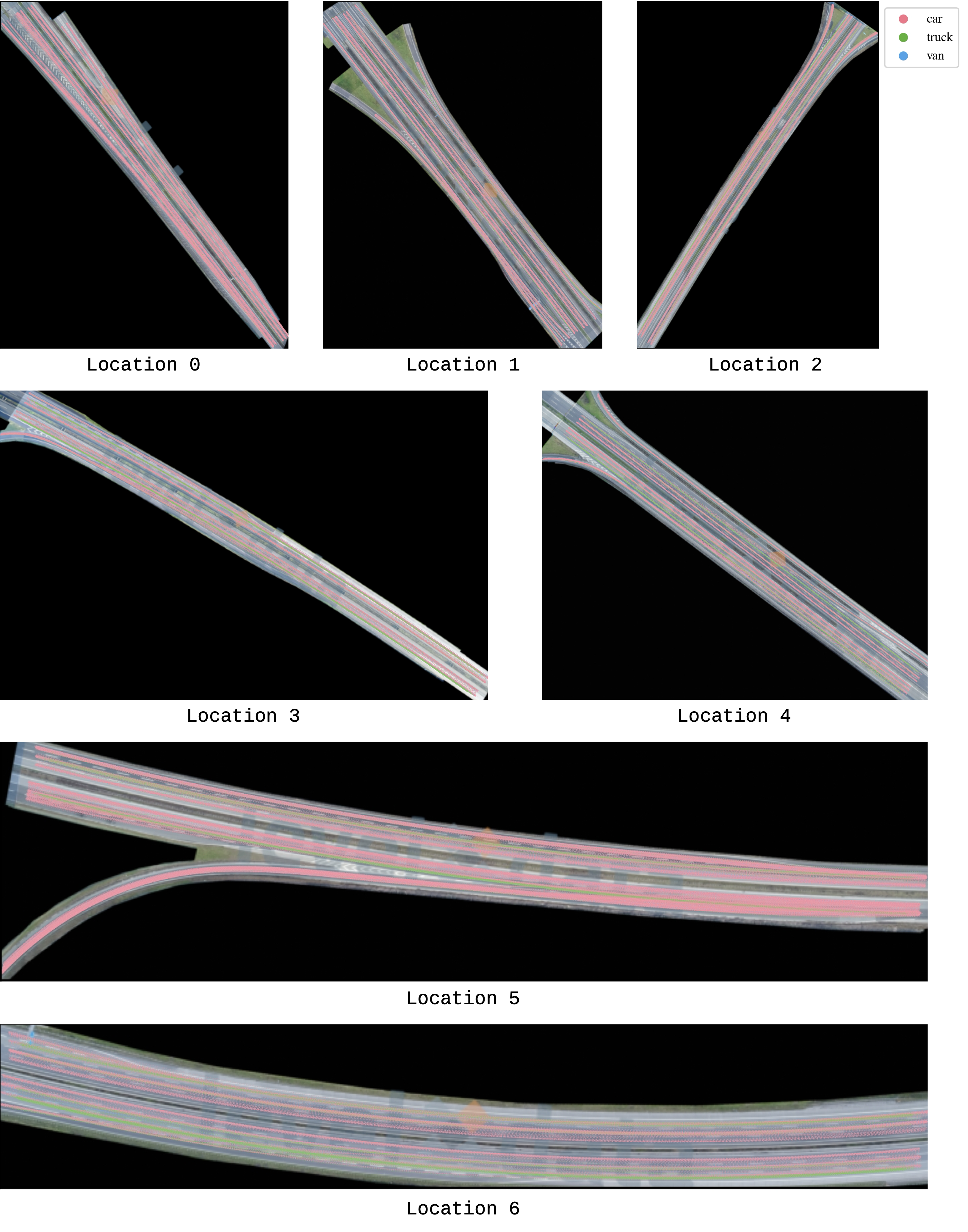
Distribution of Average Speed on Map¶

The speed heatmap exhibits a characteristic highway speed distribution. Outer lanes (leftmost) display reduced average speeds relative to inner lanes (rightmost), consistent with typical lane usage patterns. Additionally, speeds are notably lower at highway entry points, reflecting acceleration behavior as vehicles merge into the main traffic flow.

In [8]:

hide_input

for i in range(7):
    x_min = np.floor(dfs[i]["xCenter"].min())
    x_max = np.ceil(dfs[i]["xCenter"].max())
    y_min = np.floor(dfs[i]["yCenter"].min())
    y_max = np.ceil(dfs[i]["yCenter"].max())
    vx = dfs[i]["xVelocity"].to_numpy()
    vy = dfs[i]["yVelocity"].to_numpy()

    x_edges_1 = np.linspace(x_min, x_max, num=int((x_max - x_min) * 10 + 1), endpoint=True)
    y_edges_1 = np.linspace(y_min, y_max, num=int((y_max - y_min) * 10 + 1), endpoint=True)
    x_bin_1 = np.digitize(dfs[i]["xCenter"].to_numpy(), x_edges_1) - 1
    y_bin_1 = np.digitize(dfs[i]["yCenter"].to_numpy(), y_edges_1) - 1
    x_edges_2 = np.linspace(x_min, x_max, num=int((x_max - x_min) * 2 + 1), endpoint=True)
    y_edges_2 = np.linspace(y_min, y_max, num=int((y_max - y_min) * 2 + 1), endpoint=True)
    x_bin_2 = np.digitize(dfs[i]["xCenter"].to_numpy(), x_edges_2) - 1
    y_bin_2 = np.digitize(dfs[i]["yCenter"].to_numpy(), y_edges_2) - 1
    speed = np.sqrt(vx**2 + vy**2)
    heading = np.arctan(vy / vx)

    dfs[i] = dfs[i].with_columns(
        [
            pl.Series("x_bin_1", x_bin_1),
            pl.Series("y_bin_1", y_bin_1),
            pl.Series("x_bin_2", x_bin_2),
            pl.Series("y_bin_2", y_bin_2),
            pl.Series("speed (m/s)", speed),
            pl.Series("heading (radian)", heading),
        ]
    )

for i in range(7): x_min = np.floor(dfs[i]["xCenter"].min()) x_max = np.ceil(dfs[i]["xCenter"].max()) y_min = np.floor(dfs[i]["yCenter"].min()) y_max = np.ceil(dfs[i]["yCenter"].max()) vx = dfs[i]["xVelocity"].to_numpy() vy = dfs[i]["yVelocity"].to_numpy() x_edges_1 = np.linspace(x_min, x_max, num=int((x_max - x_min) * 10 + 1), endpoint=True) y_edges_1 = np.linspace(y_min, y_max, num=int((y_max - y_min) * 10 + 1), endpoint=True) x_bin_1 = np.digitize(dfs[i]["xCenter"].to_numpy(), x_edges_1) - 1 y_bin_1 = np.digitize(dfs[i]["yCenter"].to_numpy(), y_edges_1) - 1 x_edges_2 = np.linspace(x_min, x_max, num=int((x_max - x_min) * 2 + 1), endpoint=True) y_edges_2 = np.linspace(y_min, y_max, num=int((y_max - y_min) * 2 + 1), endpoint=True) x_bin_2 = np.digitize(dfs[i]["xCenter"].to_numpy(), x_edges_2) - 1 y_bin_2 = np.digitize(dfs[i]["yCenter"].to_numpy(), y_edges_2) - 1 speed = np.sqrt(vx**2 + vy**2) heading = np.arctan(vy / vx) dfs[i] = dfs[i].with_columns( [ pl.Series("x_bin_1", x_bin_1), pl.Series("y_bin_1", y_bin_1), pl.Series("x_bin_2", x_bin_2), pl.Series("y_bin_2", y_bin_2), pl.Series("speed (m/s)", speed), pl.Series("heading (radian)", heading), ] )

In [9]:

hide_input

fig = plt.figure(figsize=(6, 9))
gs = gridspec.GridSpec(4, 6, figure=fig, height_ratios=[9, 8, 6, 4])

fig.subplots_adjust(left=0.05, right=0.95, top=0.9, bottom=0.05, wspace=0.1, hspace=0.4)

positions = [(0, 0, 2), (0, 2, 4), (0, 4, 6), (1, 0, 3), (1, 3, 6), (2, 0, 6), (3, 0, 6)]

axes = []
for i in range(7):
    row, start_col, end_col = positions[i]
    ax = fig.add_subplot(gs[row, start_col:end_col])

    df_speed_heatmap = (
        dfs[i]
        .group_by(["y_bin_1", "x_bin_1"])
        .agg(pl.col("speed (m/s)").mean().alias("avg_speed"))
        .sort(["y_bin_1", "x_bin_1"])
    ).to_pandas()

    grid = df_speed_heatmap.pivot(index="y_bin_1", columns="x_bin_1", values="avg_speed")

    hm = sns.heatmap(
        grid, ax=ax, cmap="cool", cbar=False, xticklabels=False, yticklabels=False, vmin=0, vmax=60
    )

    ax.set_aspect("equal")
    ax.set_xlabel(f"Location {i}")
    ax.set_ylabel("")
    axes.append(ax)

cbar_ax = fig.add_axes([0.1, 0.94, 0.8, 0.015])
fig.colorbar(axes[-1].collections[0], cax=cbar_ax, orientation="horizontal")

plt.show()

fig = plt.figure(figsize=(6, 9)) gs = gridspec.GridSpec(4, 6, figure=fig, height_ratios=[9, 8, 6, 4]) fig.subplots_adjust(left=0.05, right=0.95, top=0.9, bottom=0.05, wspace=0.1, hspace=0.4) positions = [(0, 0, 2), (0, 2, 4), (0, 4, 6), (1, 0, 3), (1, 3, 6), (2, 0, 6), (3, 0, 6)] axes = [] for i in range(7): row, start_col, end_col = positions[i] ax = fig.add_subplot(gs[row, start_col:end_col]) df_speed_heatmap = ( dfs[i] .group_by(["y_bin_1", "x_bin_1"]) .agg(pl.col("speed (m/s)").mean().alias("avg_speed")) .sort(["y_bin_1", "x_bin_1"]) ).to_pandas() grid = df_speed_heatmap.pivot(index="y_bin_1", columns="x_bin_1", values="avg_speed") hm = sns.heatmap( grid, ax=ax, cmap="cool", cbar=False, xticklabels=False, yticklabels=False, vmin=0, vmax=60 ) ax.set_aspect("equal") ax.set_xlabel(f"Location {i}") ax.set_ylabel("") axes.append(ax) cbar_ax = fig.add_axes([0.1, 0.94, 0.8, 0.015]) fig.colorbar(axes[-1].collections[0], cax=cbar_ax, orientation="horizontal") plt.show()

¶

Distribution of Lane Change Frequency on Map¶

The figure illustrates the cumulative count of lane-changing events within each predefined grid cell on the map. Lane changes are relatively evenly distributed along the main highway lanes, while sharp increases in lane-changing activity are observed near entrances, exits, merge, and diverge areas.

In [10]:

hide_input

fig = plt.figure(figsize=(6, 9))
gs = gridspec.GridSpec(4, 6, figure=fig, height_ratios=[9, 8, 6, 4])

fig.subplots_adjust(left=0.05, right=0.95, top=0.9, bottom=0.05, wspace=0.1, hspace=0.4)

positions = [(0, 0, 2), (0, 2, 4), (0, 4, 6), (1, 0, 3), (1, 3, 6), (2, 0, 6), (3, 0, 6)]

axes = []
for i in range(7):
    row, start_col, end_col = positions[i]
    ax = fig.add_subplot(gs[row, start_col:end_col])

    df_lane_changing = dfs[i].to_pandas()
    df_lane_changing = df_lane_changing.sort_values(by=["fileId", "trackId", "frame"])
    df_lane_changing["prev_laneletId"] = df_lane_changing.groupby(["fileId", "trackId"])[
        "laneletId"
    ].shift(1)
    df_lane_changing["laneChange"] = (
        df_lane_changing["laneletId"] != df_lane_changing["prev_laneletId"]
    ).astype(int)
    first_row_mask = df_lane_changing.groupby(["fileId", "trackId"]).cumcount() == 0
    df_lane_changing.loc[first_row_mask, "laneChange"] = 0
    df_lane_changing_heatmap = (
        df_lane_changing.groupby(["y_bin_2", "x_bin_2"])["laneChange"].sum().unstack(fill_value=0)
    )
    print(
        f"Maximum lane changing in one grid (location {i}): {df_lane_changing_heatmap.to_numpy().max()}"
    )
    mask = df_lane_changing_heatmap == 0
    hm = sns.heatmap(
        df_lane_changing_heatmap,
        mask=mask,
        ax=ax,
        cmap="cool",
        cbar=False,
        xticklabels=False,
        yticklabels=False,
        vmin=0,
        vmax=400,
    )

    ax.set_aspect("equal")
    ax.set_xlabel(f"Location {i}")
    ax.set_ylabel("")
    axes.append(ax)

cbar_ax = fig.add_axes([0.1, 0.94, 0.8, 0.015])
fig.colorbar(axes[-1].collections[0], cax=cbar_ax, orientation="horizontal")

plt.show()

fig = plt.figure(figsize=(6, 9)) gs = gridspec.GridSpec(4, 6, figure=fig, height_ratios=[9, 8, 6, 4]) fig.subplots_adjust(left=0.05, right=0.95, top=0.9, bottom=0.05, wspace=0.1, hspace=0.4) positions = [(0, 0, 2), (0, 2, 4), (0, 4, 6), (1, 0, 3), (1, 3, 6), (2, 0, 6), (3, 0, 6)] axes = [] for i in range(7): row, start_col, end_col = positions[i] ax = fig.add_subplot(gs[row, start_col:end_col]) df_lane_changing = dfs[i].to_pandas() df_lane_changing = df_lane_changing.sort_values(by=["fileId", "trackId", "frame"]) df_lane_changing["prev_laneletId"] = df_lane_changing.groupby(["fileId", "trackId"])[ "laneletId" ].shift(1) df_lane_changing["laneChange"] = ( df_lane_changing["laneletId"] != df_lane_changing["prev_laneletId"] ).astype(int) first_row_mask = df_lane_changing.groupby(["fileId", "trackId"]).cumcount() == 0 df_lane_changing.loc[first_row_mask, "laneChange"] = 0 df_lane_changing_heatmap = ( df_lane_changing.groupby(["y_bin_2", "x_bin_2"])["laneChange"].sum().unstack(fill_value=0) ) print( f"Maximum lane changing in one grid (location {i}): {df_lane_changing_heatmap.to_numpy().max()}" ) mask = df_lane_changing_heatmap == 0 hm = sns.heatmap( df_lane_changing_heatmap, mask=mask, ax=ax, cmap="cool", cbar=False, xticklabels=False, yticklabels=False, vmin=0, vmax=400, ) ax.set_aspect("equal") ax.set_xlabel(f"Location {i}") ax.set_ylabel("") axes.append(ax) cbar_ax = fig.add_axes([0.1, 0.94, 0.8, 0.015]) fig.colorbar(axes[-1].collections[0], cax=cbar_ax, orientation="horizontal") plt.show()

Maximum lane changing in one grid (location 0): 549
Maximum lane changing in one grid (location 1): 732
Maximum lane changing in one grid (location 2): 771
Maximum lane changing in one grid (location 3): 454
Maximum lane changing in one grid (location 4): 648
Maximum lane changing in one grid (location 5): 405
Maximum lane changing in one grid (location 6): 482

Distribution of Speed by Trajectory Type¶

Different trajectory types exhibit peak speeds at distinct values. Cars typically demonstrate the highest average speeds, followed closely by vans, while trucks display significantly lower speeds. The speed profiles for each vehicle type remain relatively consistent across locations, suggesting that the highway scenarios represented in the exiD dataset are largely homogeneous.

In [11]:

hide_input

fig, axes = plt.subplots(7, 1, figsize=(6, 6), sharex=True)
for i in range(7):
    df_speed = dfs[i].to_pandas()

    sns.histplot(
        df_speed,
        x="speed (m/s)",
        hue="class",
        hue_order=["car", "truck", "van"],
        multiple="layer",
        palette="Set2",
        ax=axes[i],
        stat="density",
        common_norm=False,
        binwidth=0.6,
        binrange=(0, 60),
        linewidth=0,
        alpha=0.5,
        legend=(i == 0),
    )

    axes[i].set_xlim([0, 60])
    axes[i].set_ylabel(f"Location {i+1}")

fig.text(0.02, 0.5, "Probability Density", va="center", rotation="vertical")

fig.tight_layout(rect=[0.03, 0, 1, 1])
plt.show()

fig, axes = plt.subplots(7, 1, figsize=(6, 6), sharex=True) for i in range(7): df_speed = dfs[i].to_pandas() sns.histplot( df_speed, x="speed (m/s)", hue="class", hue_order=["car", "truck", "van"], multiple="layer", palette="Set2", ax=axes[i], stat="density", common_norm=False, binwidth=0.6, binrange=(0, 60), linewidth=0, alpha=0.5, legend=(i == 0), ) axes[i].set_xlim([0, 60]) axes[i].set_ylabel(f"Location {i+1}") fig.text(0.02, 0.5, "Probability Density", va="center", rotation="vertical") fig.tight_layout(rect=[0.03, 0, 1, 1]) plt.show()

Tactics2D Integration¶

This section explains how to parse and replay logs from the exiD dataset by Tactics2D.

Dataset Preparation¶

You can place the exiD dataset in any directory of your choice. However, it’s important to maintain the following folder structure for compatibility:

exiD
├── data
│   ├── 01_highway.png
│   ├── 01_recordingMeta.csv
│   ├── 01_tracks.csv
│   ├── 01_tracksMeta.csv
│   ├── ...

Class Mapping¶

The table below illustrates how classes from the exiD dataset are mapped to corresponding traffic participants in the Tactics2D framework. In this mapping, both cars and trucks from exiD are represented as the generic Vehicle class within Tactics2D.

Class	Tactics2D
car	tactics2d.participant.element.Vehicle
truck	tactics2d.participant.element.Vehicle
van	tactics2d.participant.element.Vehicle

Parse and Replay Logs¶

To parse, replay, and visualize the exiD dataset using Tactics2D, you can use the following code snippet:

In [12]:

%matplotlib notebook

import os
import numpy as np
from matplotlib.animation import FuncAnimation
from shapely.geometry import Point
from IPython.display import HTML

from tactics2d.dataset_parser import LevelXParser
from tactics2d.map.parser import OSMParser
from tactics2d.map.map_config import EXID_MAP_CONFIG
from tactics2d.sensor import BEVCamera
from tactics2d.renderer import MatplotlibRenderer

%matplotlib notebook import os import numpy as np from matplotlib.animation import FuncAnimation from shapely.geometry import Point from IPython.display import HTML from tactics2d.dataset_parser import LevelXParser from tactics2d.map.parser import OSMParser from tactics2d.map.map_config import EXID_MAP_CONFIG from tactics2d.sensor import BEVCamera from tactics2d.renderer import MatplotlibRenderer

The maps of exiD dataset are part of the official dataset. According to the data sharing protocol, Tactics2D cannot spread its maps publicly. Please apply for the dataset and maps from the official website.

In [13]:

path_dataset = "../../data/exiD/data"  # Replace with your dataset path
path_maps = "../../data/exiD_map"  # Replace with your map path
dataset_parser = LevelXParser("exiD")
map_parser = OSMParser(lanelet2=True)

path_dataset = "../../data/exiD/data" # Replace with your dataset path path_maps = "../../data/exiD_map" # Replace with your map path dataset_parser = LevelXParser("exiD") map_parser = OSMParser(lanelet2=True)

For simplicity, we revise a function from the ScenarioManager to handle the parsing and replaying of the exiD dataset:

In [14]:

def render_levelx(map_, participants, map_boundary, time_range, resolution):
    x_min, x_max, y_min, y_max = map_boundary
    x_max -= 100
    camera_position = np.array([(x_max + x_min) / 2, (y_max + y_min) / 2])
    camera = BEVCamera(id_=0, map_=map_)

    renderer = MatplotlibRenderer(
        xlim=(x_min, x_max), ylim=(y_min, y_max), resolution=resolution, auto_scale=False
    )

    fig = renderer.fig  # Use the one already created
    frame_list = list(range(time_range[0], time_range[1], 40))
    prev_road_id_set = set()
    prev_participant_id_set = set()

    def update(frame):
        nonlocal prev_road_id_set, prev_participant_id_set

        participant_ids = [pid for pid, p in participants.items() if p.is_active(frame)]

        geometry_data, prev_road_id_set, prev_participant_id_set = camera.update(
            frame,
            participants,
            participant_ids,
            prev_road_id_set,
            prev_participant_id_set,
            Point(camera_position),
        )

        renderer.update(geometry_data)
        renderer.ax.set_title(f"Frame: {frame}")

    ani = FuncAnimation(fig, update, frames=frame_list, interval=40, repeat=True)
    return ani

def render_levelx(map_, participants, map_boundary, time_range, resolution): x_min, x_max, y_min, y_max = map_boundary x_max -= 100 camera_position = np.array([(x_max + x_min) / 2, (y_max + y_min) / 2]) camera = BEVCamera(id_=0, map_=map_) renderer = MatplotlibRenderer( xlim=(x_min, x_max), ylim=(y_min, y_max), resolution=resolution, auto_scale=False ) fig = renderer.fig # Use the one already created frame_list = list(range(time_range[0], time_range[1], 40)) prev_road_id_set = set() prev_participant_id_set = set() def update(frame): nonlocal prev_road_id_set, prev_participant_id_set participant_ids = [pid for pid, p in participants.items() if p.is_active(frame)] geometry_data, prev_road_id_set, prev_participant_id_set = camera.update( frame, participants, participant_ids, prev_road_id_set, prev_participant_id_set, Point(camera_position), ) renderer.update(geometry_data) renderer.ax.set_title(f"Frame: {frame}") ani = FuncAnimation(fig, update, frames=frame_list, interval=40, repeat=True) return ani

In [15]:

participants, actual_time_range = dataset_parser.parse_trajectory(
    file=0, folder=path_dataset, time_range=(0, 10000)
)
map_ = map_parser.parse(
    file_path=os.path.join(path_maps, "exiD_0.osm"), configs=EXID_MAP_CONFIG["exiD_0"]
)

print(f"Map boundary of exiD location 0: {map_.boundary}.")

boundary = (map_.boundary[0], map_.boundary[1] + 100, map_.boundary[2], map_.boundary[3])

print(f"Map range we display: {boundary}")

ani = render_levelx(map_, participants, boundary, actual_time_range, resolution=(1000, 1000))
HTML(ani.to_html5_video())

participants, actual_time_range = dataset_parser.parse_trajectory( file=0, folder=path_dataset, time_range=(0, 10000) ) map_ = map_parser.parse( file_path=os.path.join(path_maps, "exiD_0.osm"), configs=EXID_MAP_CONFIG["exiD_0"] ) print(f"Map boundary of exiD location 0: {map_.boundary}.") boundary = (map_.boundary[0], map_.boundary[1] + 100, map_.boundary[2], map_.boundary[3]) print(f"Map range we display: {boundary}") ani = render_levelx(map_, participants, boundary, actual_time_range, resolution=(1000, 1000)) HTML(ani.to_html5_video())

Map boundary of exiD location 0: (np.float64(196.0), np.float64(654.0), np.float64(-558.0), np.float64(-22.0)).
Map range we display: (np.float64(196.0), np.float64(754.0), np.float64(-558.0), np.float64(-22.0))

Out[15]:

In the same way, we display the log in other locations in exiD.

In [16]:

hide_input

participants, actual_time_range = dataset_parser.parse_trajectory(
    file=19, folder=path_dataset, time_range=(10000, 20000)
)
map_ = map_parser.parse(
    file_path=os.path.join(path_maps, "exiD_1.osm"), configs=EXID_MAP_CONFIG["exiD_1"]
)

print(f"Map boundary of exiD location 1: {map_.boundary}.")

boundary = (map_.boundary[0], map_.boundary[1] + 100, map_.boundary[2], map_.boundary[3])

print(f"Map range we display: {boundary}")

ani = render_levelx(map_, participants, boundary, actual_time_range, resolution=(1000, 1000))
HTML(ani.to_html5_video())

participants, actual_time_range = dataset_parser.parse_trajectory( file=19, folder=path_dataset, time_range=(10000, 20000) ) map_ = map_parser.parse( file_path=os.path.join(path_maps, "exiD_1.osm"), configs=EXID_MAP_CONFIG["exiD_1"] ) print(f"Map boundary of exiD location 1: {map_.boundary}.") boundary = (map_.boundary[0], map_.boundary[1] + 100, map_.boundary[2], map_.boundary[3]) print(f"Map range we display: {boundary}") ani = render_levelx(map_, participants, boundary, actual_time_range, resolution=(1000, 1000)) HTML(ani.to_html5_video())

Map boundary of exiD location 1: (np.float64(261.0), np.float64(607.0), np.float64(-430.0), np.float64(-23.0)).
Map range we display: (np.float64(261.0), np.float64(707.0), np.float64(-430.0), np.float64(-23.0))

Out[16]:

In [17]:

hide_input

participants, actual_time_range = dataset_parser.parse_trajectory(
    file=39, folder=path_dataset, time_range=(20000, 30000)
)
map_ = map_parser.parse(
    file_path=os.path.join(path_maps, "exiD_2.osm"), configs=EXID_MAP_CONFIG["exiD_2"]
)

print(f"Map boundary of exiD location 2: {map_.boundary}.")

boundary = (map_.boundary[0], map_.boundary[1] + 100, map_.boundary[2], map_.boundary[3])

print(f"Map range we display: {boundary}")

ani = render_levelx(map_, participants, boundary, actual_time_range, resolution=(1000, 1000))
HTML(ani.to_html5_video())

participants, actual_time_range = dataset_parser.parse_trajectory( file=39, folder=path_dataset, time_range=(20000, 30000) ) map_ = map_parser.parse( file_path=os.path.join(path_maps, "exiD_2.osm"), configs=EXID_MAP_CONFIG["exiD_2"] ) print(f"Map boundary of exiD location 2: {map_.boundary}.") boundary = (map_.boundary[0], map_.boundary[1] + 100, map_.boundary[2], map_.boundary[3]) print(f"Map range we display: {boundary}") ani = render_levelx(map_, participants, boundary, actual_time_range, resolution=(1000, 1000)) HTML(ani.to_html5_video())

Map boundary of exiD location 2: (np.float64(529.0), np.float64(892.0), np.float64(-628.0), np.float64(-148.0)).
Map range we display: (np.float64(529.0), np.float64(992.0), np.float64(-628.0), np.float64(-148.0))

Out[17]:

In [18]:

hide_input

participants, actual_time_range = dataset_parser.parse_trajectory(
    file=53, folder=path_dataset, time_range=(30000, 40000)
)
map_ = map_parser.parse(
    file_path=os.path.join(path_maps, "exiD_3.osm"), configs=EXID_MAP_CONFIG["exiD_3"]
)

print(f"Map boundary of exiD location 3: {map_.boundary}.")

boundary = (map_.boundary[0], map_.boundary[1] + 100, map_.boundary[2], map_.boundary[3])

print(f"Map range we display: {boundary}")

ani = render_levelx(map_, participants, boundary, actual_time_range, resolution=(1000, 1000))
HTML(ani.to_html5_video())

participants, actual_time_range = dataset_parser.parse_trajectory( file=53, folder=path_dataset, time_range=(30000, 40000) ) map_ = map_parser.parse( file_path=os.path.join(path_maps, "exiD_3.osm"), configs=EXID_MAP_CONFIG["exiD_3"] ) print(f"Map boundary of exiD location 3: {map_.boundary}.") boundary = (map_.boundary[0], map_.boundary[1] + 100, map_.boundary[2], map_.boundary[3]) print(f"Map range we display: {boundary}") ani = render_levelx(map_, participants, boundary, actual_time_range, resolution=(1000, 1000)) HTML(ani.to_html5_video())

Map boundary of exiD location 3: (np.float64(76.0), np.float64(588.0), np.float64(-353.0), np.float64(-10.0)).
Map range we display: (np.float64(76.0), np.float64(688.0), np.float64(-353.0), np.float64(-10.0))

Out[18]:

In [19]:

hide_input

participants, actual_time_range = dataset_parser.parse_trajectory(
    file=73, folder=path_dataset, time_range=(40000, 50000)
)
map_ = map_parser.parse(
    file_path=os.path.join(path_maps, "exiD_5.osm"), configs=EXID_MAP_CONFIG["exiD_5"]
)

print(f"Map boundary of exiD location 5: {map_.boundary}.")

boundary = (map_.boundary[0], map_.boundary[1] + 100, map_.boundary[2], map_.boundary[3])

print(f"Map range we display: {boundary}")

ani = render_levelx(map_, participants, boundary, actual_time_range, resolution=(2000, 1000))
HTML(ani.to_html5_video())

participants, actual_time_range = dataset_parser.parse_trajectory( file=73, folder=path_dataset, time_range=(40000, 50000) ) map_ = map_parser.parse( file_path=os.path.join(path_maps, "exiD_5.osm"), configs=EXID_MAP_CONFIG["exiD_5"] ) print(f"Map boundary of exiD location 5: {map_.boundary}.") boundary = (map_.boundary[0], map_.boundary[1] + 100, map_.boundary[2], map_.boundary[3]) print(f"Map range we display: {boundary}") ani = render_levelx(map_, participants, boundary, actual_time_range, resolution=(2000, 1000)) HTML(ani.to_html5_video())

Map boundary of exiD location 5: (np.float64(124.0), np.float64(695.0), np.float64(-334.0), np.float64(-143.0)).
Map range we display: (np.float64(124.0), np.float64(795.0), np.float64(-334.0), np.float64(-143.0))

Out[19]:

In [20]:

hide_input

participants, actual_time_range = dataset_parser.parse_trajectory(
    file=78, folder=path_dataset, time_range=(50000, 60000)
)
map_ = map_parser.parse(
    file_path=os.path.join(path_maps, "exiD_6.osm"), configs=EXID_MAP_CONFIG["exiD_6"]
)

print(f"Map boundary of exiD location 6: {map_.boundary}.")

boundary = (map_.boundary[0], map_.boundary[1] + 100, map_.boundary[2], map_.boundary[3])

print(f"Map range we display: {boundary}")

ani = render_levelx(map_, participants, boundary, actual_time_range, resolution=(2000, 1000))
HTML(ani.to_html5_video())

participants, actual_time_range = dataset_parser.parse_trajectory( file=78, folder=path_dataset, time_range=(50000, 60000) ) map_ = map_parser.parse( file_path=os.path.join(path_maps, "exiD_6.osm"), configs=EXID_MAP_CONFIG["exiD_6"] ) print(f"Map boundary of exiD location 6: {map_.boundary}.") boundary = (map_.boundary[0], map_.boundary[1] + 100, map_.boundary[2], map_.boundary[3]) print(f"Map range we display: {boundary}") ani = render_levelx(map_, participants, boundary, actual_time_range, resolution=(2000, 1000)) HTML(ani.to_html5_video())

Map boundary of exiD location 6: (np.float64(129.0), np.float64(653.0), np.float64(-225.0), np.float64(-137.0)).
Map range we display: (np.float64(129.0), np.float64(753.0), np.float64(-225.0), np.float64(-137.0))

Out[20]:

Appendix: Data Format¶

Note

This is a backup copy of the official documentation , provided here for reference purposes only.

The dataset includes measurement data extracted from one or more recording sites (locations) in the data directory as well as map files per location in the maps directory (if part of the dataset). Data and maps can be associated using a recording's location id. The data for each location is split into multiple continuous recordings.

In total four files are provided for each recording:

• An image of the recorded road section (XX_background.png)
• A csv file describing the recording location (XX_recordingsMeta.csv)
• A csv file containing an overview of recorded vehicle and VRU tracks (XX_tracksMeta.csv)
• A csv file for the tracks' trajectories (XX_tracks.csv) These files are created for each recording to ensure easy handling of the data.

In addition the following map data for each recording location are provided:

• Lanelet2 maps (.osm)
• ASAM OpenDrive maps (.xodr)
• 3D scene (.osgb & .fbx)

In the following, the dataset format and especially the meaning of every column is explained in detail.

Please note that we summarize pedestrians, bicyclists and motorcycles to vulnerable road users (VRUs) in the following tables.

Image of the Road Section¶

For each recording a georeferenced image of the road section is added.The image is based on the recording itself by removing all moving vehicles through filtering. Additionally the resolution of the image was reduced.

Recording Meta Information¶

This file contains metadata for each recording. The metadata provides a general overview, e.g. of the time of recording, the road section considered and the total number of objects tracked.

Name	Description	Unit
recordingId	The id of the recording. Every recording has a unique id.	[-]
locationId	The id of the recording location.	[-]
frameRate	The frame rate which was used to record the video.	[hz]
speedLimit	The speed limit of the driving lanes. In all recordings, the speed limit is the same for every driving lane.	[m/s]
weekday	The weekday the recording was done.	[-]
startTime	The hour at which the recording was started	[hh]
duration	The duration of the recording.	[s]
numTracks	The number of objects tracked.	[-]
numVehicles	The number of vehicles tracked.	[-]
numVrus	The number of vulnerable road users (VRUs) tracked.	[-]
latLocation	Rough latitude coordinates of recording location. Not to be confused with UTM coordinates!	[deg]
lonLocation	Rough longitude coordinates of recording location. Not to be confused with UTM coordinates!	[deg]
xUtmOrigin	X value of UTM coordinate of origin of the local coordinate system for this recording location. Add this to xCenter to get UTM coordinates.	[m]
yUtmOrigin	Y value of UTM coordinate of origin of the local coordinate system for this recording location. Add this to yCenter to get UTM coordinates.	[m]
orthoPxToMeter	Scale factor from ortho image pixels to UTM meters. This value is needed for visualization.	[m/px]
exportVersion	Version of data format. (may be missing in some datasets)	[-]

Track Meta Information¶

This file contains an overview of all tracks.

The purpose of this file is to allow filtering tracks e.g. by class.

Name	Description	Unit
recordingId	The id of the recording. Every recording has a unique id.	[-]
trackId	The id of the track. The ids are assigned in ascending order for each recording.	[-]
initialFrame	The frame in which the track starts.	[-]
finalFrame	The frame in which the track ends.	[-]
numFrames	The total lifetime in frames.	[-]
width	The width of the tracked object. This property is set to zero for VRUs.	[m]
length	The length of the tracked object. This property is set to zero for VRUs.	[m]
class	The class of the tracked object.	[-]

Tracks¶

This file contains all time dependent values for each track. Information such as current position, velocity and acceleration.

Name	Description	Unit
recordingId	The id of the recording. Every recording has a unique id.	[-]
trackId	The track's id. The ids are assigned in ascending order for each recording.	[-]
frame	The frame for which the information are given.	[-]
trackLifetime	The current age of the track at this frame.	[-]
xCenter	The x position of the object's centroid in the local coordinate system. Add xUtmOrigin to get UTM coordinates.	[m]
yCenter	The y position of the object's centroid in the local coordinate system. Add yUtmOrigin to get UTM coordinates.	[m]
heading	The heading in the local coordinate system.	[deg]
width	The width of the object. This property is set to zero for VRUs.	[m]
length	The height of the object. This property is set to zero for VRUs.	[m]
xVelocity	The velocity in x-axis direction in the local coordinate system.	[m/s]
yVelocity	The velocity in y-axis direction in the local coordinate system.	[m/s]
xAcceleration	The acceleration in x-axis direction in the local coordinate system.	[m/s²]
yAcceleration	The acceleration in y-axis direction in the local coordinate system.	[m/s²]
lonVelocity	The longitudinal velocity.	[m/s]
latVelocity	The lateral velocity.	[m/s]
lonAcceleration	The longitudinal acceleration.	[m/s²]
latAcceleration	The lateral acceleration.	[m/s²]
traveledDistance	The accumulated distance covered by the track up to this point in time.	[m]
latLaneCenterOffset	Lateral offset of the vehicle's centroid to the closest point on the centerline of the lanelet the vehicle is currently driving in. Semicolon-separated list with values for each lanelet the vehicle is currently in. (*)	[m]
laneWidth	Width of the lane at the current centroid position of the vehicle. Semicolon-separated list with values for each lanelet the vehicle is currently in. (*)	[m]
laneletId	Semicolon-separated list of the IDs of the lanelets the vehicle is currently driving in according to the Lanelet2 map. Determined by the vehicle's centroid position. (*)	[-]
laneChange	Whether the lane was changed in lateral direction. First frame, in which the centroid is in the new lane.	[m]
lonLaneletPos	Length of the segments of the centerline from the start of the lanelet to the closest point on the centerline from the vehicle's centroid. Semicolon-separated list with values for each lanelet the vehicle is currently in. (*)	[m]
laneletLength	Length of the complete centerline of the lanelet the vehicle is currently driving in. Semicolon-separated list with values for each lanelet the vehicle is currently in. (*)	[m]
leadDHW	Distance Headway from the front bumper of the current vehicle to the rear bumper of its lead vehicle (default value: -1).	[m]
leadDV	Relative velocity between the current vehicle and its lead vehicle. Positive if the current vehicle is faster than lead (default value: -1000).	[m/s]
leadTHW	Time Headway from the front bumper of the current vehicle to the rear bumper of its lead vehicle (default value: -1).	[s]
leadTTC	Time-to-Collision from the front bumper of the current vehicle to the rear bumper of its lead vehicle (default value: -1).	[s]
leadId	The ID of the lead vehicle in the same lane (default value: -1). (**) This and the following surrounding vehicle IDs are best visualized using the drone-dataset-tools.	[-]
rearId	The ID of the rear vehicle in the same lane (default value: -1). (**)	[-]
leftLeadId	The ID of the lead vehicle in the left adjacent lane in travel direction or in one of its further left adjacent lanes (default value: -1). (**)	[-]
leftRearId	The ID of the rear vehicle in the left adjacent lane in travel direction or in one of its further left adjacent lanes (default value: -1). (**)	[-]
leftAlongsideId	Semicolon-separated list of the IDs of the alongside vehicles (with longitudinal overlap) to the left of the vehicle in travel direction or in one of its further left adjacent lanes (default value: empty). (**)	[-]
rightLeadId	The ID of the lead vehicle in the right adjacent lane in travel direction or in one of its further right adjacent lanes (default value: -1). (**)	[-]
rightRearId	The ID of the rear vehicle in the right adjacent lane in travel direction or in on of its further right adjacent lanes (default value: -1). (**)	[-]
rightAlongsideId	Semicolon-separated list of the IDs of the alongside vehicles (with longitudinal overlap) to the right of the vehicle in travel direction or in one of its further left adjacent lanes (default value: empty). (**)	[-]

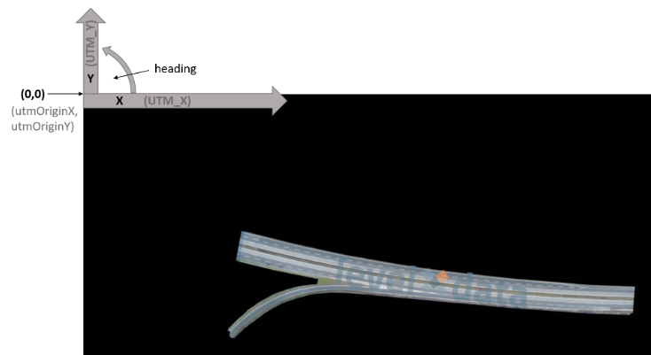
Coordinate System¶

The global coordinate system used is the UTM coordinate system, as we geo-referenced our data. For easier handling of data of the same intersection in different recordings, we introduced a local UTM-like coordinate system.

The only difference is, that the origin (0, 0) is very close to the recorded road section and the same for all recordings at each location.

To transform positions into the global UTM coordinate system, just add xUtmOrigin and yUtmOrigin to all positions.

The local coordinate system looks as follows: The horizontal axis is the x-axis, which grows to the right.

The vertical axis is the y-axis, which grows upwards.

The heading is calcuated as in the UTM coordinate system.

Finally, we use SI units only.