CitySim¶

About¶

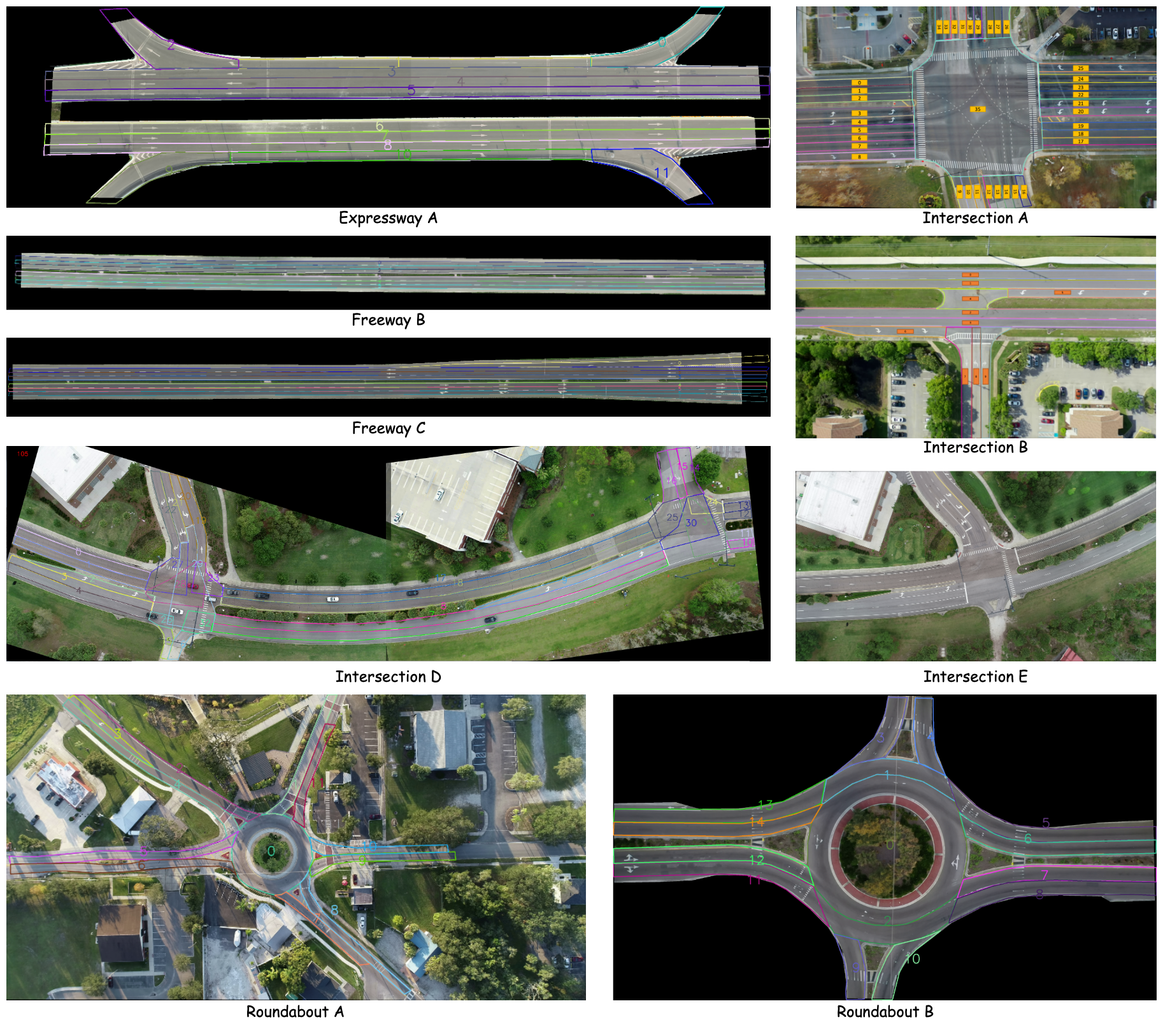
While the original paper lists the locations shown in the following table, the actual dataset we obtained includes a different set of locations:

Expressway A
Freeway B
Freeway C
Intersection A
Intersection B
Intersection D
Intersection E
Roundabout A
Roundabout B

The data analysis in the subsequent sections will be based on this actual dataset we received.

ID	Location	Location type	Drone height (m)	FPS	Recording resolution (pixel)	Recording length (min)
1	Expressway A	Weaving segment	120	30	5120×2880	120
2	Freeway B	Basic segment	320	30	5120×2880	60
3	Freeway C	Merge/diverge segment	320	30	5120×2880	60
4	Expressway D	Merge/diverge segment	120	30	3840×2160	60
5	Intersection A	Signalized intersection	120	30	3840×2160	120
6	Intersection B	Signalized intersection	120	30	3840×2160	120
7	Intersection C	Signalized intersection	120	30	4096×2160	120
8	Intersection D	Signalized intersection	120	30	3840×2160	120
9	Intersection E	Signalized intersection	120	30	3840×2160	120
10	Intersection F	Stop-control intersection	120	30	3840×2160	120
11	Intersection G	Control-free intersectiona	120	30	3840×2160	60
12	Intersection H	Control-free intersection	120	30	3840×2160	60

How to Apply¶

To apply for access to the full dataset, please send the official dataset holder a request form to this email: citysim.ucfsst@gmail.com

Citation¶

@article{zheng2024citysim,
  title={CitySim: A drone-based vehicle trajectory dataset for safety-oriented research and digital twins},
  author={Zheng, Ou and Abdel-Aty, Mohamed and Yue, Lishengsa and Abdelraouf, Amr and Wang, Zijin and Mahmoud, Nada},
  journal={Transportation research record},
  volume={2678},
  number={4},
  pages={606--621},
  year={2024},
  publisher={SAGE Publications Sage CA: Los Angeles, CA}
}

Data Analysis¶

This part is independently conducted by Tactics2D.

Overview of Available Locations¶

Here is a visualization of the available locations in the actual dataset.

In [1]:

hide_input

Copied!





%matplotlib inline
import warnings

warnings.filterwarnings("ignore")

import logging

logging.basicConfig(level=logging.WARNING)

import os
import glob

import polars as pl
import numpy as np
import matplotlib as mpl
import matplotlib.gridspec as gridspec
import matplotlib.pyplot as plt
import seaborn as sns
%matplotlib inline
import warnings

warnings.filterwarnings("ignore")

import logging

logging.basicConfig(level=logging.WARNING)

import os
import glob

import polars as pl
import numpy as np
import matplotlib as mpl
import matplotlib.gridspec as gridspec
import matplotlib.pyplot as plt
import seaborn as sns

In [2]:

hide_input

Copied!





# Setting up parameters for matplotlib
mpl.rcParams.update(
    {
        "figure.dpi": 200,  # 200 for high quality
        "font.family": "DejaVu Sans Mono",
        "font.size": 6,
        "font.stretch": "semi-expanded",
        "animation.html": "jshtml",
        "animation.embed_limit": 5000,
        "axes.edgecolor": "black",
        "axes.linewidth": 0.8,
        "axes.grid": True,
        "grid.color": "#cccccc",
        "axes.facecolor": "white",
    }
)
sns.set_palette("Set2")
# Setting up parameters for matplotlib
mpl.rcParams.update(
    {
        "figure.dpi": 200,  # 200 for high quality
        "font.family": "DejaVu Sans Mono",
        "font.size": 6,
        "font.stretch": "semi-expanded",
        "animation.html": "jshtml",
        "animation.embed_limit": 5000,
        "axes.edgecolor": "black",
        "axes.linewidth": 0.8,
        "axes.grid": True,
        "grid.color": "#cccccc",
        "axes.facecolor": "white",
    }
)
sns.set_palette("Set2")

In [3]:

hide_input

Copied!





root_path = "../../data/CitySim"
csv_paths = {}

for dir_path, dir_names, file_names in os.walk(root_path):
    if os.path.basename(dir_path) == "Trajectories":
        csv_files = glob.glob(os.path.join(dir_path, "*.csv"))
        csv_paths[dir_path] = [os.path.basename(f) for f in csv_files]
root_path = "../../data/CitySim"
csv_paths = {}

for dir_path, dir_names, file_names in os.walk(root_path):
    if os.path.basename(dir_path) == "Trajectories":
        csv_files = glob.glob(os.path.join(dir_path, "*.csv"))
        csv_paths[dir_path] = [os.path.basename(f) for f in csv_files]

Distribution of Average Speed on Map¶

The speed of vehicles exhibits significant variation across different locations. Highways, for instance, display an average speed of over 30 m/s, while roundabouts show a much lower average speed of around 10 m/s. According to the speed heatmap, speed records are only available for lanes, and the dataset does not provide labels for the types of trajectories. Therefore, we have to assume that the CitySim dataset includes trajectory information solely for vehicle types, with no further categorization of trajectory types.

In [4]:

hide_input

Copied!





locations = [
    "Expressway A",
    "Freeway B",
    "Freeway C",
    "Intersection A",
    "Intersection B",
    "Intersection D",
    "Intersection E",
    "Roundabout A",
    "Roundabout B",
]
positions = [
    (0, 1, 0, 4),
    (1, 2, 0, 4),
    (2, 3, 0, 4),
    (0, 1, 4, 6),
    (1, 3, 4, 6),
    (3, 4, 0, 4),
    (3, 4, 4, 6),
    (4, 5, 0, 3),
    (4, 5, 3, 6),
]
locations = [
    "Expressway A",
    "Freeway B",
    "Freeway C",
    "Intersection A",
    "Intersection B",
    "Intersection D",
    "Intersection E",
    "Roundabout A",
    "Roundabout B",
]
positions = [
    (0, 1, 0, 4),
    (1, 2, 0, 4),
    (2, 3, 0, 4),
    (0, 1, 4, 6),
    (1, 3, 4, 6),
    (3, 4, 0, 4),
    (3, 4, 4, 6),
    (4, 5, 0, 3),
    (4, 5, 3, 6),
]

In [5]:

hide_input

Copied!





fig = plt.figure(figsize=(6, 6))
gs = gridspec.GridSpec(5, 6, figure=fig, height_ratios=[1.3, 0.4, 0.4, 1.3, 2.6])

fig.subplots_adjust(left=0.05, right=0.95, top=0.9, bottom=0.05, wspace=0.1, hspace=0.4)

axes = []

for i, location in enumerate(locations):
    start_row, end_row, start_col, end_col = positions[i]
    ax = fig.add_subplot(gs[start_row:end_row, start_col:end_col])
    df = pl.DataFrame()

    for dir_path in csv_paths.keys():
        if location in dir_path:
            dir_path = dir_path
            csv_files = csv_paths[dir_path]
            break

    for csv_file in csv_files:
        df_csv = pl.read_csv(os.path.join(dir_path, csv_file))
        df_csv = df_csv.select(["carCenterX", "carCenterY", "speed"])
        df = pl.concat([df, df_csv])

    x_min = np.floor(df["carCenterX"].min())
    x_max = np.ceil(df["carCenterX"].max())
    y_min = np.floor(df["carCenterY"].min())
    y_max = np.ceil(df["carCenterY"].max())
    x_edges = np.linspace(x_min, x_max, num=int((x_max - x_min) * 10 + 1), endpoint=True)
    y_edges = np.linspace(y_min, y_max, num=int((y_max - y_min) * 10 + 1), endpoint=True)
    x_bin = np.digitize(df["carCenterX"].to_numpy(), x_edges) - 1
    y_bin = np.digitize(df["carCenterY"].to_numpy(), y_edges) - 1
    speed_m_per_s = 0.447 * df["speed"]  # convert speed's unit from mile/hour to m/s

    df = df.with_columns(
        [
            pl.Series("x_bin", x_bin),
            pl.Series("y_bin", y_bin),
            pl.Series("speed (m/s)", speed_m_per_s),
        ]
    )

    df_speed_heatmap = (
        df.group_by(["y_bin", "x_bin"])
        .agg(pl.col("speed (m/s)").mean().alias("avg_speed"))
        .sort(["y_bin", "x_bin"])
    ).to_pandas()

    grid = df_speed_heatmap.pivot(index="y_bin", columns="x_bin", values="avg_speed")

    hm = sns.heatmap(
        grid, ax=ax, cmap="cool", cbar=False, xticklabels=False, yticklabels=False, vmin=0, vmax=40
    )

    ax.set_aspect("equal")
    ax.set_xlabel(location)
    ax.set_ylabel("")
    axes.append(ax)

cbar_ax = fig.add_axes([0.1, 0.94, 0.8, 0.015])
fig.colorbar(axes[-1].collections[0], cax=cbar_ax, orientation="horizontal")
fig = plt.figure(figsize=(6, 6))
gs = gridspec.GridSpec(5, 6, figure=fig, height_ratios=[1.3, 0.4, 0.4, 1.3, 2.6])

fig.subplots_adjust(left=0.05, right=0.95, top=0.9, bottom=0.05, wspace=0.1, hspace=0.4)

axes = []

for i, location in enumerate(locations):
    start_row, end_row, start_col, end_col = positions[i]
    ax = fig.add_subplot(gs[start_row:end_row, start_col:end_col])
    df = pl.DataFrame()

    for dir_path in csv_paths.keys():
        if location in dir_path:
            dir_path = dir_path
            csv_files = csv_paths[dir_path]
            break

    for csv_file in csv_files:
        df_csv = pl.read_csv(os.path.join(dir_path, csv_file))
        df_csv = df_csv.select(["carCenterX", "carCenterY", "speed"])
        df = pl.concat([df, df_csv])

    x_min = np.floor(df["carCenterX"].min())
    x_max = np.ceil(df["carCenterX"].max())
    y_min = np.floor(df["carCenterY"].min())
    y_max = np.ceil(df["carCenterY"].max())
    x_edges = np.linspace(x_min, x_max, num=int((x_max - x_min) * 10 + 1), endpoint=True)
    y_edges = np.linspace(y_min, y_max, num=int((y_max - y_min) * 10 + 1), endpoint=True)
    x_bin = np.digitize(df["carCenterX"].to_numpy(), x_edges) - 1
    y_bin = np.digitize(df["carCenterY"].to_numpy(), y_edges) - 1
    speed_m_per_s = 0.447 * df["speed"]  # convert speed's unit from mile/hour to m/s

    df = df.with_columns(
        [
            pl.Series("x_bin", x_bin),
            pl.Series("y_bin", y_bin),
            pl.Series("speed (m/s)", speed_m_per_s),
        ]
    )

    df_speed_heatmap = (
        df.group_by(["y_bin", "x_bin"])
        .agg(pl.col("speed (m/s)").mean().alias("avg_speed"))
        .sort(["y_bin", "x_bin"])
    ).to_pandas()

    grid = df_speed_heatmap.pivot(index="y_bin", columns="x_bin", values="avg_speed")

    hm = sns.heatmap(
        grid, ax=ax, cmap="cool", cbar=False, xticklabels=False, yticklabels=False, vmin=0, vmax=40
    )

    ax.set_aspect("equal")
    ax.set_xlabel(location)
    ax.set_ylabel("")
    axes.append(ax)

cbar_ax = fig.add_axes([0.1, 0.94, 0.8, 0.015])
fig.colorbar(axes[-1].collections[0], cax=cbar_ax, orientation="horizontal")

Out[5]:

<matplotlib.colorbar.Colorbar at 0x7caf636bcf70>

No description has been provided for this image

Distribution of Lane Change Frequency on Map¶

The heatmap suggests that lane changes are relatively infrequent in this dataset, even in highway scenarios where such behavior is typically more common.

In [6]:

hide_input

Copied!





fig = plt.figure(figsize=(6, 6))
gs = gridspec.GridSpec(5, 6, figure=fig, height_ratios=[1.3, 0.4, 0.4, 1.3, 2.6])

fig.subplots_adjust(left=0.05, right=0.95, top=0.9, bottom=0.05, wspace=0.1, hspace=0.4)

axes = []

for i, location in enumerate(locations):
    start_row, end_row, start_col, end_col = positions[i]
    ax = fig.add_subplot(gs[start_row:end_row, start_col:end_col])
    df = pl.DataFrame()

    for dir_path in csv_paths.keys():
        if location in dir_path:
            dir_path = dir_path
            csv_files = csv_paths[dir_path]
            break

    for csv_file in csv_files:
        df_csv = pl.read_csv(os.path.join(dir_path, csv_file))
        df_csv = df_csv.select(["carId", "carCenterX", "carCenterY", "laneId", "frameNum"])
        df_csv = df_csv.with_columns(pl.lit(csv_file).alias("fileId"))
        df = pl.concat([df, df_csv])

    x_min = np.floor(df["carCenterX"].min())
    x_max = np.ceil(df["carCenterX"].max())
    y_min = np.floor(df["carCenterY"].min())
    y_max = np.ceil(df["carCenterY"].max())
    x_edges = np.linspace(x_min, x_max, num=int((x_max - x_min) * 2 + 1), endpoint=True)
    y_edges = np.linspace(y_min, y_max, num=int((y_max - y_min) * 2 + 1), endpoint=True)
    x_bin = np.digitize(df["carCenterX"].to_numpy(), x_edges) - 1
    y_bin = np.digitize(df["carCenterY"].to_numpy(), y_edges) - 1

    df = df.with_columns([pl.Series("x_bin", x_bin), pl.Series("y_bin", y_bin)])

    df_lane_changing = df.to_pandas()
    df_lane_changing = df_lane_changing.sort_values(by=["fileId", "carId", "frameNum"])
    df_lane_changing["prev_laneId"] = df_lane_changing.groupby(["fileId", "carId"])["laneId"].shift(
        1
    )
    df_lane_changing["laneChange"] = (
        df_lane_changing["laneId"] != df_lane_changing["prev_laneId"]
    ).astype(int)
    first_row_mask = df_lane_changing.groupby(["fileId", "carId"]).cumcount() == 0
    df_lane_changing.loc[first_row_mask, "laneChange"] = 0
    df_lane_changing_heatmap = (
        df_lane_changing.groupby(["y_bin", "x_bin"])["laneChange"].sum().unstack(fill_value=0)
    )
    print(
        f"Maximum lane changing in one grid ({location}): {df_lane_changing_heatmap.to_numpy().max()}"
    )

    mask = df_lane_changing_heatmap == 0
    hm = sns.heatmap(
        df_lane_changing_heatmap,
        mask=mask,
        ax=ax,
        cmap="cool",
        cbar=False,
        xticklabels=False,
        yticklabels=False,
        vmin=0,
        vmax=10,
    )

    ax.set_aspect("equal")
    ax.set_xlabel(location)
    ax.set_ylabel("")
    axes.append(ax)

cbar_ax = fig.add_axes([0.1, 0.94, 0.8, 0.015])
fig.colorbar(axes[-1].collections[0], cax=cbar_ax, orientation="horizontal")
fig = plt.figure(figsize=(6, 6))
gs = gridspec.GridSpec(5, 6, figure=fig, height_ratios=[1.3, 0.4, 0.4, 1.3, 2.6])

fig.subplots_adjust(left=0.05, right=0.95, top=0.9, bottom=0.05, wspace=0.1, hspace=0.4)

axes = []

for i, location in enumerate(locations):
    start_row, end_row, start_col, end_col = positions[i]
    ax = fig.add_subplot(gs[start_row:end_row, start_col:end_col])
    df = pl.DataFrame()

    for dir_path in csv_paths.keys():
        if location in dir_path:
            dir_path = dir_path
            csv_files = csv_paths[dir_path]
            break

    for csv_file in csv_files:
        df_csv = pl.read_csv(os.path.join(dir_path, csv_file))
        df_csv = df_csv.select(["carId", "carCenterX", "carCenterY", "laneId", "frameNum"])
        df_csv = df_csv.with_columns(pl.lit(csv_file).alias("fileId"))
        df = pl.concat([df, df_csv])

    x_min = np.floor(df["carCenterX"].min())
    x_max = np.ceil(df["carCenterX"].max())
    y_min = np.floor(df["carCenterY"].min())
    y_max = np.ceil(df["carCenterY"].max())
    x_edges = np.linspace(x_min, x_max, num=int((x_max - x_min) * 2 + 1), endpoint=True)
    y_edges = np.linspace(y_min, y_max, num=int((y_max - y_min) * 2 + 1), endpoint=True)
    x_bin = np.digitize(df["carCenterX"].to_numpy(), x_edges) - 1
    y_bin = np.digitize(df["carCenterY"].to_numpy(), y_edges) - 1

    df = df.with_columns([pl.Series("x_bin", x_bin), pl.Series("y_bin", y_bin)])

    df_lane_changing = df.to_pandas()
    df_lane_changing = df_lane_changing.sort_values(by=["fileId", "carId", "frameNum"])
    df_lane_changing["prev_laneId"] = df_lane_changing.groupby(["fileId", "carId"])["laneId"].shift(
        1
    )
    df_lane_changing["laneChange"] = (
        df_lane_changing["laneId"] != df_lane_changing["prev_laneId"]
    ).astype(int)
    first_row_mask = df_lane_changing.groupby(["fileId", "carId"]).cumcount() == 0
    df_lane_changing.loc[first_row_mask, "laneChange"] = 0
    df_lane_changing_heatmap = (
        df_lane_changing.groupby(["y_bin", "x_bin"])["laneChange"].sum().unstack(fill_value=0)
    )
    print(
        f"Maximum lane changing in one grid ({location}): {df_lane_changing_heatmap.to_numpy().max()}"
    )

    mask = df_lane_changing_heatmap == 0
    hm = sns.heatmap(
        df_lane_changing_heatmap,
        mask=mask,
        ax=ax,
        cmap="cool",
        cbar=False,
        xticklabels=False,
        yticklabels=False,
        vmin=0,
        vmax=10,
    )

    ax.set_aspect("equal")
    ax.set_xlabel(location)
    ax.set_ylabel("")
    axes.append(ax)

cbar_ax = fig.add_axes([0.1, 0.94, 0.8, 0.015])
fig.colorbar(axes[-1].collections[0], cax=cbar_ax, orientation="horizontal")

Maximum lane changing in one grid (Expressway A): 30
Maximum lane changing in one grid (Freeway B): 4
Maximum lane changing in one grid (Freeway C): 11
Maximum lane changing in one grid (Intersection A): 102
Maximum lane changing in one grid (Intersection B): 2
Maximum lane changing in one grid (Intersection D): 5
Maximum lane changing in one grid (Intersection E): 29
Maximum lane changing in one grid (Roundabout A): 18
Maximum lane changing in one grid (Roundabout B): 10

Out[6]:

<matplotlib.colorbar.Colorbar at 0x7caf5df0eec0>

Distribution of Speed by Location¶

The distribution of vehicle speeds varies across different locations, but there is no clear correlation between scenario types and specific speed distribution patterns.

In [7]:

hide_input

Copied!





fig, axes = plt.subplots(9, 1, figsize=(6, 8), sharex=True, sharey=True)

for i, location in enumerate(locations):
    df = pl.DataFrame()

    for dir_path in csv_paths.keys():
        if location in dir_path:
            dir_path = dir_path
            csv_files = csv_paths[dir_path]
            break

    for csv_file in csv_files:
        df_csv = pl.read_csv(os.path.join(dir_path, csv_file))
        df_csv = df_csv.select(["speed"])
        df = pl.concat([df, df_csv])

    df_speed = df.to_pandas()
    df_speed["speed (m/s)"] = df_speed["speed"] * 0.447

    sns.histplot(
        df_speed,
        x="speed (m/s)",
        palette="Set2",
        ax=axes[i],
        stat="density",
        log_scale=(False, True),
        common_norm=False,
        binwidth=1.0,
        binrange=(0, 50),
        linewidth=0,
        alpha=0.5,
        legend=(i == 0),
    )

    axes[i].set_xlim([0, 50])
    axes[i].set_ylabel(location, fontsize=6)
    axes[i].set_yscale("log")

axes[-1].set_xlabel("speed (m/s)")
fig.text(0.02, 0.5, "Probability Density", va="center", rotation="vertical")

fig.tight_layout(rect=[0.04, 0, 1, 1])
plt.show()
fig, axes = plt.subplots(9, 1, figsize=(6, 8), sharex=True, sharey=True)

for i, location in enumerate(locations):
    df = pl.DataFrame()

    for dir_path in csv_paths.keys():
        if location in dir_path:
            dir_path = dir_path
            csv_files = csv_paths[dir_path]
            break

    for csv_file in csv_files:
        df_csv = pl.read_csv(os.path.join(dir_path, csv_file))
        df_csv = df_csv.select(["speed"])
        df = pl.concat([df, df_csv])

    df_speed = df.to_pandas()
    df_speed["speed (m/s)"] = df_speed["speed"] * 0.447

    sns.histplot(
        df_speed,
        x="speed (m/s)",
        palette="Set2",
        ax=axes[i],
        stat="density",
        log_scale=(False, True),
        common_norm=False,
        binwidth=1.0,
        binrange=(0, 50),
        linewidth=0,
        alpha=0.5,
        legend=(i == 0),
    )

    axes[i].set_xlim([0, 50])
    axes[i].set_ylabel(location, fontsize=6)
    axes[i].set_yscale("log")

axes[-1].set_xlabel("speed (m/s)")
fig.text(0.02, 0.5, "Probability Density", va="center", rotation="vertical")

fig.tight_layout(rect=[0.04, 0, 1, 1])
plt.show()

Tactics2D Integration¶

This section explains how to parse and replay logs from the highD dataset by CitySim.

Dataset Preparation¶

You can place the CitySim dataset in any directory of your choice. The folder and file structure of CitySim is in a mess so here we give up to provide a sample for it. Please specify the folder path and file names in any way you like.

Class Mapping¶

All the traffic participants in CitySim are vehicles, mapping to tactics2d.participant.element.Vehicle in Tactics2D's framework.

Parse and Replay Logs¶

To parse, replay, and visualize the CitySim dataset using Tactics2D, you can use the following code snippet:

In [8]:

Copied!





%matplotlib notebook

import os
import numpy as np
from matplotlib.animation import FuncAnimation
from shapely.geometry import Point
from IPython.display import HTML

from tactics2d.dataset_parser import CitySimParser
from tactics2d.map.parser import OSMParser
from tactics2d.sensor import BEVCamera
from tactics2d.renderer import MatplotlibRenderer
from tactics2d.map.element import Map
%matplotlib notebook

import os
import numpy as np
from matplotlib.animation import FuncAnimation
from shapely.geometry import Point
from IPython.display import HTML

from tactics2d.dataset_parser import CitySimParser
from tactics2d.map.parser import OSMParser
from tactics2d.sensor import BEVCamera
from tactics2d.renderer import MatplotlibRenderer
from tactics2d.map.element import Map

In [9]:

Copied!

dataset_path = "../../data/CitySim"  # Replace with your dataset path
dataset_parser = CitySimParser()
map_parser = OSMParser()
dataset_path = "../../data/CitySim"  # Replace with your dataset path
dataset_parser = CitySimParser()
map_parser = OSMParser()

In [10]:

Copied!





def render_citysim(map_, participants, map_boundary, time_range):
    x_min, x_max, y_min, y_max = map_boundary
    camera_position = np.array([0, 0])
    camera = BEVCamera(id_=0, map_=map_, perception_range=150)

    renderer = MatplotlibRenderer(xlim=(x_min, x_max), ylim=(y_min, y_max), resolution=(2000, 800))

    fig = renderer.fig  # Use the one already created

    frame_list = []
    for i in range(time_range[1]):
        i = int(i * 1000 / 30)
        if i >= time_range[1]:
            break
        elif i < time_range[0]:
            continue
        frame_list.append(i)

    prev_road_id_set = set()
    prev_participant_id_set = set()

    def update(frame):
        nonlocal prev_road_id_set, prev_participant_id_set

        participant_ids = [pid for pid, p in participants.items() if p.is_active(frame)]

        geometry_data, prev_road_id_set, prev_participant_id_set = camera.update(
            frame,
            participants,
            participant_ids,
            prev_road_id_set,
            prev_participant_id_set,
            Point(camera_position),
        )

        renderer.update(geometry_data, camera_position)
        renderer.ax.set_title(f"Frame: {frame}")

    ani = FuncAnimation(fig, update, frames=frame_list, interval=30, repeat=True)
    return ani
def render_citysim(map_, participants, map_boundary, time_range):
    x_min, x_max, y_min, y_max = map_boundary
    camera_position = np.array([0, 0])
    camera = BEVCamera(id_=0, map_=map_, perception_range=150)

    renderer = MatplotlibRenderer(xlim=(x_min, x_max), ylim=(y_min, y_max), resolution=(2000, 800))

    fig = renderer.fig  # Use the one already created

    frame_list = []
    for i in range(time_range[1]):
        i = int(i * 1000 / 30)
        if i >= time_range[1]:
            break
        elif i < time_range[0]:
            continue
        frame_list.append(i)

    prev_road_id_set = set()
    prev_participant_id_set = set()

    def update(frame):
        nonlocal prev_road_id_set, prev_participant_id_set

        participant_ids = [pid for pid, p in participants.items() if p.is_active(frame)]

        geometry_data, prev_road_id_set, prev_participant_id_set = camera.update(
            frame,
            participants,
            participant_ids,
            prev_road_id_set,
            prev_participant_id_set,
            Point(camera_position),
        )

        renderer.update(geometry_data, camera_position)
        renderer.ax.set_title(f"Frame: {frame}")

    ani = FuncAnimation(fig, update, frames=frame_list, interval=30, repeat=True)
    return ani

In [11]:

Copied!





participants, actual_time_range = dataset_parser.parse_trajectory(
    file="IntersectionA-01.csv",
    folder=os.path.join(dataset_path, "Intersection A (Signalized Intersection)/Trajectories"),
    time_range=(0, 5000),
)

map_ = Map()

boundary = (-10, 160, -20, 100)
print(f"Map range of Intersection A (Signalized Intersection) we display: {boundary}")

ani = render_citysim(map_, participants, boundary, actual_time_range)
HTML(ani.to_html5_video())
participants, actual_time_range = dataset_parser.parse_trajectory(
    file="IntersectionA-01.csv",
    folder=os.path.join(dataset_path, "Intersection A (Signalized Intersection)/Trajectories"),
    time_range=(0, 5000),
)

map_ = Map()

boundary = (-10, 160, -20, 100)
print(f"Map range of Intersection A (Signalized Intersection) we display: {boundary}")

ani = render_citysim(map_, participants, boundary, actual_time_range)
HTML(ani.to_html5_video())

Map range of Intersection A (Signalized Intersection) we display: (-10, 160, -20, 100)

Out[11]:

In [12]:

hide_input

Copied!





participants, actual_time_range = dataset_parser.parse_trajectory(
    file="IntersectionD-01.csv",
    folder=os.path.join(dataset_path, "Intersection D (Permissive Left Turn Phasing)/Trajectories"),
    time_range=(3000, 10000),
)

map_ = Map()

boundary = (0, 270, 0, 85)
print(f"Map range of Intersection D (Permissive Left Turn Phasing) we display: {boundary}")

ani = render_citysim(map_, participants, boundary, actual_time_range)
HTML(ani.to_html5_video())
participants, actual_time_range = dataset_parser.parse_trajectory(
    file="IntersectionD-01.csv",
    folder=os.path.join(dataset_path, "Intersection D (Permissive Left Turn Phasing)/Trajectories"),
    time_range=(3000, 10000),
)

map_ = Map()

boundary = (0, 270, 0, 85)
print(f"Map range of Intersection D (Permissive Left Turn Phasing) we display: {boundary}")

ani = render_citysim(map_, participants, boundary, actual_time_range)
HTML(ani.to_html5_video())

Map range of Intersection D (Permissive Left Turn Phasing) we display: (0, 270, 0, 85)

Out[12]:

In [13]:

hide_input

Copied!





participants, actual_time_range = dataset_parser.parse_trajectory(
    file="IntersectionE-01.csv",
    folder=os.path.join(dataset_path, "Intersection E (Permissive Left Turn Phasing)/Trajectories"),
    time_range=(0, 10000),
)

map_ = Map()

boundary = (10, 150, 0, 70)
print(f"Map range of Intersection E (Permissive Left Turn Phasing) we display: {boundary}")

ani = render_citysim(map_, participants, boundary, actual_time_range)
HTML(ani.to_html5_video())
participants, actual_time_range = dataset_parser.parse_trajectory(
    file="IntersectionE-01.csv",
    folder=os.path.join(dataset_path, "Intersection E (Permissive Left Turn Phasing)/Trajectories"),
    time_range=(0, 10000),
)

map_ = Map()

boundary = (10, 150, 0, 70)
print(f"Map range of Intersection E (Permissive Left Turn Phasing) we display: {boundary}")

ani = render_citysim(map_, participants, boundary, actual_time_range)
HTML(ani.to_html5_video())

Map range of Intersection E (Permissive Left Turn Phasing) we display: (10, 150, 0, 70)

Out[13]:

In [14]:

hide_input

Copied!





participants, actual_time_range = dataset_parser.parse_trajectory(
    file="RoundaboutA-01.csv",
    folder=os.path.join(dataset_path, "Roundabout A (Single Lane)/Trajectories"),
    time_range=(0, 10000),
)

map_ = Map()

boundary = (20, 180, 20, 130)
print(f"Map range of Roundabout A (Single Lane) we display: {boundary}")

ani = render_citysim(map_, participants, boundary, actual_time_range)
HTML(ani.to_html5_video())
participants, actual_time_range = dataset_parser.parse_trajectory(
    file="RoundaboutA-01.csv",
    folder=os.path.join(dataset_path, "Roundabout A (Single Lane)/Trajectories"),
    time_range=(0, 10000),
)

map_ = Map()

boundary = (20, 180, 20, 130)
print(f"Map range of Roundabout A (Single Lane) we display: {boundary}")

ani = render_citysim(map_, participants, boundary, actual_time_range)
HTML(ani.to_html5_video())

Map range of Roundabout A (Single Lane) we display: (20, 180, 20, 130)

Out[14]:

In [15]:

Copied!





participants, actual_time_range = dataset_parser.parse_trajectory(
    file="RoundaboutB-01.csv",
    folder=os.path.join(dataset_path, "Roundabout B (Multiple Lanes)/Trajectories"),
    time_range=(0, 10000),
)

map_ = Map()

boundary = (-5, 150, 20, 85)
print(f"Map range of Roundabout B (Multiple Lanes) we display: {boundary}")

ani = render_citysim(map_, participants, boundary, actual_time_range)
HTML(ani.to_html5_video())
participants, actual_time_range = dataset_parser.parse_trajectory(
    file="RoundaboutB-01.csv",
    folder=os.path.join(dataset_path, "Roundabout B (Multiple Lanes)/Trajectories"),
    time_range=(0, 10000),
)

map_ = Map()

boundary = (-5, 150, 20, 85)
print(f"Map range of Roundabout B (Multiple Lanes) we display: {boundary}")

ani = render_citysim(map_, participants, boundary, actual_time_range)
HTML(ani.to_html5_video())

Map range of Roundabout B (Multiple Lanes) we display: (-5, 150, 20, 85)

Out[15]:

Appendix: Data Format¶

Note

This is a backup copy of the official documentation , provided here for reference purposes only.

Trajectory¶

The UCF SST CitySim dataset contains vehicle trajectories captured using drone videos. The videos were captured at 30 frames per second. Each row in the trajectory dataset represents a vehicle waypoint at a single frame in the video. Additionally, the dataset describes the rotation-aware vehicle bounding box in each row.

The following table describes the trajectory CSV columns and states their respective units.

Name	Description	Unit
frameNum	Frame number of the vehicle waypoint captured at 30 frames per second	-
carId	Vehicle unique identifier that remains consistent for all vehicle waypoints across the entire video	-
carCenterX	Pixel x-coordinate of vehicle bounding box center point	Pixel
carCenterY	Pixel y-coordinate of vehicle bounding box center point	Pixel
headX	Pixel x-coordinate of vehicle bounding box front center point	Pixel
headY	Pixel y-coordinate of vehicle bounding box front center point	Pixel
tailX	Pixel x-coordinate of vehicle bounding box rear center point	Pixel
tailY	Pixel y-coordinate of vehicle bounding box rear center point	Pixel
boundingBox1X	Pixel x-coordinate of vehicle bounding box vertex 1	Pixel
boundingBox1Y	Pixel y-coordinate of vehicle bounding box vertex 1	Pixel
boundingBox2X	Pixel x-coordinate of vehicle bounding box vertex 2	Pixel
boundingBox2Y	Pixel y-coordinate of vehicle bounding box vertex 2	Pixel
boundingBox3X	Pixel x-coordinate of vehicle bounding box vertex 3	Pixel
boundingBox3Y	Pixel y-coordinate of vehicle bounding box vertex 3	Pixel
boundingBox4X	Pixel x-coordinate of vehicle bounding box vertex 4	Pixel
boundingBox4Y	Pixel y-coordinate of vehicle bounding box vertex 4	Pixel
carCenterXft	X-coordinate of vehicle bounding box center point in feet	Feet
carCenterYft	Y-coordinate of vehicle bounding box center point in feet	Feet
headXft	X-coordinate of vehicle bounding box front center point in feet	Feet
headYft	Y-coordinate of vehicle bounding box front center point in feet	Feet
tailXft	X-coordinate of vehicle bounding box rear center point in feet	Feet
tailYft	Y-coordinate of vehicle bounding box rear center point in feet	Feet
boundingBox1Xft	X -coordinate of vehicle bounding box vertex 1 in feet	Feet
boundingBox1Yft	Y -coordinate of vehicle bounding box vertex 1 in feet	Feet
boundingBox2Xft	X -coordinate of vehicle bounding box vertex 2 in feet	Feet
boundingBox2Yft	Y -coordinate of vehicle bounding box vertex 2 in feet	Feet
boundingBox3Xft	X -coordinate of vehicle bounding box vertex 3 in feet	Feet
boundingBox3Yft	Y -coordinate of vehicle bounding box vertex 3 in feet	Feet
boundingBox4Xft	X-coordinate of vehicle bounding box vertex 4 in feet	Feet
boundingBox4Yft	Y -coordinate of vehicle bounding box vertex 4 in feet	Feet
carCenterLat*	Global latitude of vehicle bounding box center point	Degrees
carCenterLon*	Global longitude of vehicle bounding box center point	Degrees
headLat*	Global latitude of vehicle bounding box front center point	Degrees
headLon*	Global longitude of vehicle bounding box front center point	Degrees
tailLat*	Global latitude of vehicle bounding box rear center point	Degrees
tailLon*	Global longitude of vehicle bounding box rear center point	Degrees
boundingBox1Lat*	Global latitude of vehicle bounding box vertex 1	Degrees
boundingBox1Lon*	Global longitude of vehicle bounding box vertex 1	Degrees
boundingBox2Lat*	Global latitude of vehicle bounding box vertex 1	Degrees
boundingBox2Lon*	Global longitude of vehicle bounding box vertex 1	Degrees
boundingBox3Lat*	Global latitude of vehicle bounding box vertex 1	Degrees
boundingBox3Lon*	Global longitude of vehicle bounding box vertex 1	Degrees
boundingBox4Lat*	Global latitude of vehicle bounding box vertex 1	Degrees
boundingBox4Lon*	Global longitude of vehicle bounding box vertex 1	Degrees
speed	Vehicle waypoint speed	Miles per Hour
heading	Vehicle waypoint heading relative to the global North	Degrees
course	Vehicle waypoint heading relative to the image coordinate X-axis	Degrees
laneId	Waypoint lane number according to the supplementary lane map	-

\Only provided for US-based locations*

X/Y-Coordinate System¶

The pixel coordinate system is displayed in the image below.

Vehicle Point Features¶

The vehicle center, head, tail, and bounding box vertices locations are described in figure below.

Bounding box point 1 describes the front right vehicle corner
Bounding box point 2 describes the rear right vehicle corner
Bounding box point 3 describes the rear left vehicle corner
Bounding box point 4 describes the front left vehicle corner

Lane IDs¶

A lane map file (lanes.png) is provided for each location to describe the lane numbers.

Base Map¶

Apart from the trajectory data, the CitySim dataset also provides simulation model for the corresponding location. The simulation model contains road network for microscopic traffic simulation software SUMO and automated driving software CARLA, which are both open-source simulators. The road network is built based on GIS data, and 3D high-fidelity architectures are embedded for the CARLA base map. Driving behavior model can be calibrated using the trajectories to produce realistic traffic flow in SUMO, and the calibrated model can be used for microscopic safety analysis or signal optimization. The CARLA base map enables researchers to conduct automated driving research including perception, CAV control in mixed traffic, etc.

Sumo¶

Sumo is an open-source microscopic traffic simulation software that provides powerful functions for simulating traffic flow. The Sumo model released in the dataset contains the road network file (.net.xml file) of the video location and its surrounding vicinity.

CARLA¶

CARLA is an open-source automated driving simulator built on Unreal Engine 4. The maps can be imported to CARLA to generate a digital world of the video location. It enables the researchers to conduct automated driving study including sensor simulation and CAV control algorithm, etc.

Signal Timing¶

The signal data CSV file provides event level data. Each record in the signal data represents a change in one of the signals. The data is represented by eight different digits that corresponds to different signal phases at an intersection. The eight digits show whether the signal phase is red (r), yellow (y), or green (g). Furthermore, the event start time and duration were calculated based on the start frame and end frame corresponding to the recorded videos and trajectory data. The following table describes the signal CSV file columns and their respective units.

Name	Description	Unit
startFrame	Signal event start frame	-
eventDuration	Signal event duration in seconds	Seconds
SBL	Southbound left turn signal phase (‘r’: red, ‘y’: yellow, ‘g’: green)	-
SBT	Southbound through signal phase (‘r’: red, ‘y’: yellow, ‘g’: green)	-
WBL	Westbound left turn signal phase (‘r’: red, ‘y’: yellow, ‘g’: green)	-
WBT	Westbound through signal phase (‘r’: red, ‘y’: yellow, ‘g’: green)	-
NBL	Northbound left turn signal phase (‘r’: red, ‘y’: yellow, ‘g’: green)	-
NBT	Northbound through signal phase (‘r’: red, ‘y’: yellow, ‘g’: green)	-
EBL	Eastbound left turn signal phase (‘r’: red, ‘y’: yellow, ‘g’: green)	-
EBT	Eastbound through signal phase (‘r’: red, ‘y’: yellow, ‘g’: green)	-

Signal Labels¶

A signal image file (signals.png) file is provided for each signalized intersection location to label the signals in the intersection.

Metadata¶

The metadata CSV file contains information about the drone video recordings used to extract the vehicle trajectories. The following table describes the metadata CSV file columns and their respective units.

Name	Description	Unit
fileName	File name	-
frameSizeX	Pixel x-coordinate frame size	Pixel
frameSizeY	Pixel y-coordinate frame size	Pixel
recordingFrameRate	Frame rate of the drone video used to extract the trajectories	Frames Per Second
totalFrames	Total number of frames in the file	-
recordingTime	Recording time of the file (hh:mm)	-
duration	Duration of the file	Seconds

Supplementary Material¶

Each location contains 2 supplementary images: background.png and lanes.png. Signalized intersection locations additionally contain a signals.png file.

The background.png image is an aerial shot of the location with all the vehicles removed. It can be used for visualization purposes.

The lanes.png file describe the laneId values used in the trajectory CSV files.

The signals.png file describe the signals in the intersection.